객관식 시험 자료의 사후 분석 - 고부담 시험 모니터링 및 개선: AMEE Guide No. 66 (Med Teach, 2012)
Post-examination interpretation of objective test data: Monitoring and improving the quality of high-stakes examinations: AMEE Guide No. 66
MOHSEN TAVAKOL & REG DENNICK

서론
Introduction
시험 과정의 결과는 형식적으로, 피드백의 형태로, 또는 총괄적으로 수행에 대한 공식적인 판단으로 학생들에게 전달된다. 분명히, 학생과 대중의 요구를 충족시키는 출력을 생산하기 위해서는, 프로세스에 대한 입력을 정의, 모니터링 및 제어할 필요가 있다. 고전적 시험 이론(CTT)은 시험 후 분석에 대한 input이 학생의 관찰된 지식 및 역량에 영향을 미칠 수 있는 측정 오류의 원천을 포함하고 있다고 가정한다. 측정 오류의 원인은 테스트 구성, 관리, 점수 매기기 및 성능 해석에서 도출된다. 예를 들어, 지식 기반 문항 간의 품질 차이, 평가자 간의 차이, 후보 간의 차이, 목표 구조 임상 검사(OSCE) 내의 표준화된 환자(SP) 간의 차이 등이 있다.
The output of the examination process is transferred to students either formatively, in the form of feedback, or summatively, as a formal judgement on performance. Clearly, to produce an output which fulfils the needs of students and the public, it is necessary to define, monitor and control the inputs to the process. Classical Test Theory (CTT) assumes that inputs to post-examination analysis contain sources of measurement error that can influence the student's observed scores of knowledge and competencies. Sources of measurement error is derived from test construction, administration, scoring and interpretation of performance. For example;
- quality variation among knowledge-based questions,
- differences between raters,
- differences between candidates and variation between standardised patients (SPs) within an Objective Structured Clinical Examination (OSCE).
고부담 검사의 품질을 향상시키기 위해 오류를 최소화하고 가능하면 제거해야 한다. CTT는 측정 오류의 출처를 최소화하거나 제거하면 관찰된 점수가 실제 점수에 근접할 것으로 가정한다. [신뢰성]은 검정의 측정 오차 양을 보여주는 핵심 추정치입니다. 간단한 해석은 신뢰성은 시험 자체와 그 자체의 상관관계라는 것이다. 이 상관 관계를 제곱하여 100을 곱하고 100에서 빼면 검정의 오차 백분율이 표시됩니다. 예를 들어, 시험의 신뢰도가 0.80이면 점수에 36%의 오차 분산(랜덤 오차)이 있습니다. 신뢰도 추정치가 증가할수록 오류에 기인하는 시험 점수의 비율이 감소합니다. 반대로 오차의 양이 증가하면 신뢰도 추정치는 감소합니다(Nunly & Bernstein).
To improve the quality of high-stakes examinations, errors should be minimised and, if possible, eliminated. CTT assumes that minimising or eliminating sources of measurement errors will cause the observed score to approach the true score. Reliability is the key estimate showing the amount of measurement error in a test. A simple interpretation is that reliability is the correlation of the test with itself; squaring this correlation, multiplying it by 100 and subtracting from 100 gives the percentage error in the test. For example, if an examination has a reliability of 0.80, there is 36% error variance (random error) in the scores. As the estimate of reliability increases, the fraction of a test score that is attributable to error will decrease. Conversely, if the amount of error increases, reliability estimates will decrease (Nunnally & Bernstein ).
일부 의과대학은 OSCE 검사를 모니터링하고 개선하기 위해 신뢰성 검사 및 항목 분석과 같은 정신계량학적 방법을 채택했지만(Lawson; Iramaneerat 등), 일반성 이론 및 래쉬 모델링과 같은 고급 정신계량학적 방법의 사용은 아직 널리 보급되지 않았다.
Although some medical schools have adopted psychometric methods such as reliability testing and item analysis to monitor and improve OSCE examination (Lawson ; Iramaneerat et al. ), the use of advanced psychometric methods such as generalisability theory and Rasch modelling has yet to become widespread.
따라서 이 가이드의 목적은 몇 가지 예를 사용하여 전통적인 및 고급 심리측정법의 사용과 해석을 설명하는 것이다. 궁극적으로 독자들은 자신의 시험 데이터와 함께 이러한 방법을 사용하는 것을 고려할 것을 권장한다. 우리는 다른 곳(Tavakol & Dennick)에서 SPSS를 사용하여 객관적인 테스트에서 검사 후 데이터를 생성하는 방법을 설명했으므로, 이 기사에서는 이러한 방법에 대해 논의하지 않을 것이다. 객관적 테스트와 OSCE의 검사 후 데이터에 대한 전통적인 해석으로 시작한 후 현대 심리 측정 방법의 적용을 살펴볼 것이다. 우리는 후속 검사를 개선하기 위한 방법을 예시하기 위해 시뮬레이션 데이터를 사용할 것이다.
Therefore, the objective of this Guide is to illustrate the use and interpretation of traditional and advanced psychometric methods using several examples. Ultimately, readers are encouraged to consider using these methods with their own exam data. We have explained how to generate post-examination data from objective tests using SPSS elsewhere (Tavakol & Dennick ), and therefore we will not discuss these methods in this article. We shall begin with the traditional interpretation of post-exam data from objective tests and OSCEs and then look at the application of modern psychometric methods. We will use simulated data to exemplify methods for improving subsequent examinations.
기본 사후검사 결과 해석
Interpretation of basic post-examination results
개별 질문
Individual questions
[기술 분석]은 시험의 원시 데이터를 요약하고 표시하는 첫 번째 단계입니다. 각 질문에 대한 분포 빈도는 누락된 질문의 수와 추측 행동의 패턴을 즉시 보여준다. 예를 들어, 문항에 누락된 응답이 식별되지 않은 경우, 이는 학생들이 좋은 지식을 가지고 있거나 일부 질문에 대해 추측하고 있었음을 시사한다. 반대로, 누락된 문제 응답이 있는 경우, 이는 시험을 완료하기에 부적절한 시간, 특히 어려운 시험 또는 부정적인 표시가 사용되는 것일 수 있습니다.
A descriptive analysis is the first step in summarising and presenting the raw data of an examination. A distribution frequency for each question immediately shows up the number of missing questions and the patterns of guessing behaviour. For example, if there were no missing question responses identified, this would suggest that students either had good knowledge or were guessing for some questions. Conversely, if there were missing question responses, this might be either an indication of an inadequate time for completing the examination, a particularly hard exam or negative marking is being used (Stone & Yeh ; Reeve et al. ).
시험 문제의 평균과 분산은 우리에게 각 문제에 대한 중요한 정보를 제공할 수 있다. 이분법 문항의 평균은 0점 또는 1점으로 p로 표시된 정답 학생의 비율과 같다.
- 이분법 문항의 [분산]은 문제 정답자 비율(p)에 오답자 비율(q)을 곱하여 계산한다.
- 표준 편차(SD)를 얻기 위해, 우리는 단지 p × q의 제곱근을 구한다.
예를 들어, 객관식 시험에서 300명의 학생이 1번 문제를 맞혔고 100명의 학생이 1번 문제를 틀렸을 경우, 1번 문제의 p 값은 0.75(300/400)와 같으며, 분산과 SD 값은 각각 0.18(0.75 x 0.25)과 0.42가 됩니다.
The means and variances of test questions can provide us with important information about each question. The mean of a dichotomous question, scored either 0 or 1, is equal to the proportion of students who answer correctly, denoted by p.
- The variance of a dichotomous question is calculated from the proportion of students who answer a question correctly (p) multiplied by those who answer the question incorrectly (q).
- To obtain the standard deviation (SD), we merely take the square root of p × q.
For example, if in an objective test, 300 students answered Question 1 correctly and 100 students answered it incorrectly, the p value for Question 1 will be equal to 0.75 (300/400), and the variance and SD will be 0.18 (0.75 × 0.25) and 0.42

SD는 주어진 질문 내에서 변동 또는 분산의 척도로 유용하다. SD가 낮으면 문제가 너무 쉬우거나 너무 어렵다는 것을 나타냅니다. 예를 들어, 위의 예에서 SD가 낮다는 것은 항목이 너무 쉽다는 것을 나타냅니다. 문제 1의 항목 난이도(0.75)와 낮은 항목 SD를 고려할 때 대부분의 학생들이 정답에 관심을 기울였기 때문에 항목에 대한 응답이 분산되지 않았다고 결론 내릴 수 있다. 평균이 분포의 중심에 있는 질문의 변동성이 높을 경우 질문이 유용할 수 있습니다.
respectively. The SD is useful as a measure of variation or dispersion within a given question. A low SD indicates that the question is either too easy or too hard. For example, in the above example, the SD is low indicating that the item is too easy. Given the item difficulty of Question 1 (0.75) and a low item SD, one can conclude that responses to item was not dispersed (there is little variability on the question) as most students paid attention to the correct response. If the question had a high variability with a mean at the centre of distribution, the question might be useful.
총 수행능력
Total performance
각 문항별 평균과 SD를 구한 뒤 각 문항별 학생별 정답 합계를 구한 뒤 전체 수행의 평균과 SD를 계산하는 기존 수행분석을 할 수 있다. SPSS를 사용하여 히스토그램을 만들면 특정 검정의 표시 분포를 이해할 수 있습니다. 학생들의 점수는 정규 분포를 따르거나 왼쪽이나 오른쪽으로 치우치거나 직사각형 모양으로 분포할 수 있다. 그림 1(a)은 양의 치우친 분포를 보여줍니다. 이것은 단순히 대부분의 학생들이 낮은 점수에서 중간 점수를 가지고 있고 소수의 학생들은 상대적으로 높은 점수를 받았다는 것을 보여준다. 양의 치우침 분포에서는 모수와 중위수가 평균보다 크므로 대부분의 학생들에게 문제가 어려웠음을 나타냅니다. 그림 1(b)은 학생들의 점수가 음으로 치우친 분포를 보여준다. 이것은 대부분의 학생들이 중간에서 높은 점수를 받았고 소수의 학생들은 상대적으로 낮은 점수를 받았다는 것을 보여준다. 음으로 치우친 분포에서 모수와 중위수가 평균보다 작다는 것은 대부분의 학생들이 문제가 쉬웠음을 나타냅니다.
After obtaining the mean and SD for each question, the test can be subjected to conventional performance analysis where the sum of correct responses of each student for each item is obtained and then the mean and SD of the total performance are calculated. Creating a histogram using SPSS allows us to understand the distribution of marks on a given test. Students’ marks can take either a normal distribution or may be skewed to the left or right or distributed in a rectangular shape. Figure 1(a) illustrates a positively skewed distribution. This simply shows that most students have a low-to-moderate mark and a few students received a relatively high mark in the tail. In a positively skewed distribution, the mode and the median are greater than the mean indicating that the questions were hard for most students. Figure 1(b) shows a negatively skewed distribution of students’ marks. This shows that most students have a moderate-to-high mark and a few students received relatively a low mark in the tail. In a negatively skewed distribution, the mode and the median are less than the mean indicating that the questions were easy for most students.
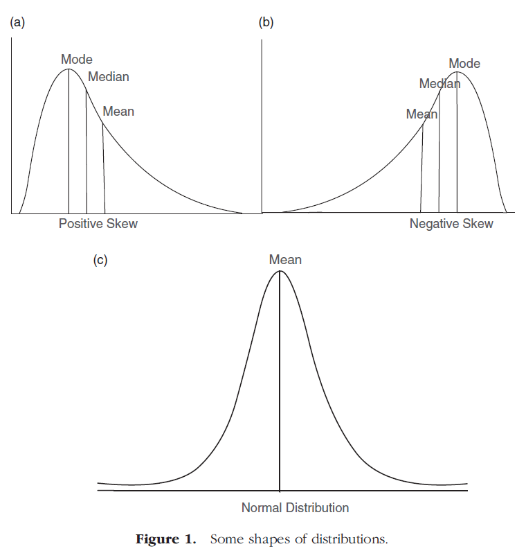
그림 1(c)은 대칭 분포 곡선의 중심에 분포된 대부분의 표시를 보여준다. 이것은 절반의 학생들이 평균보다 높은 점수를 받았고 절반의 학생들이 평균보다 낮은 점수를 받았다는 것을 의미한다. 이 경우 평균, 모드 및 중위수는 동일합니다. 이 정보를 바탕으로 모드, 중위 또는 평균에 SD의 추정치를 더하지 않으면 시험이 어려운지 쉬운지 판단하기 어렵다. 우리는 다른 곳에서 SPSS를 사용하여 이러한 통계를 계산하는 방법을 설명했습니다.
Figure 1(c) shows most marks distributed in the centre of a symmetrical distribution curve. This means that half the students scored greater than the mean and half less than mean. The mean, mode and median are identical in this situation. Based on this information, it is hard to judge whether the exam is hard or easy unless we obtain differences between the mode, median or mean plus an estimate of the SD. We have explained how to compute these statistics using SPSS elsewhere (Tavakol & Dennick ; Tavakol & Dennick 2012).
예를 들어, 그림 2의 두 분포를 고려해 볼 것을 요청합니다. 그림 2는 두 시험에서 학생들의 모의 점수를 나타냅니다.
As an example, we would ask you to consider the two distributions in Figure 2, which represent simulated marks of students in two examinations.

두 마크 분포 모두 평균이 50이지만 다른 패턴을 보입니다. A시험은 20점 이하와 90점 이상으로 점수가 다양하다. 반면에 B시험은 어느 한 극단에서나 거의 학생들이 보이지 않는다. 이 정보를 이용하여 A검사는 B검사에 비해 이질적이고 B검사는 A검사에 비해 균질하다고 할 수 있다.
Both the mark distributions have a mean of 50, but show a different pattern. Examination A has a wide range of marks, with some below 20 and some above 90. Examination B, on the other hand, shows few students at either extreme. Using this information, we can say that Examination A is more heterogeneous than Examination B and that Examination B is more homogenous than Examination A.
시험 데이터를 더 잘 해석하기 위해서는 각 분포에 대한 SD를 구해야 합니다. 예를 들어, 두 시험의 평균 점수가 67.0이고 각각 6.0과 3.0의 다른 SD를 사용하는 경우, 3.0의 SD를 사용하는 검사는 6.0의 SD를 사용하는 검사보다 더 균질하고 따라서 성능을 측정하는 데 더 일관성이 있다고 말할 수 있습니다. SD의 가치에 대한 추가적인 해석은 학생들의 점수가 평균에서 얼마나 벗어난지를 보여주는가 하는 것이다. 이것은 단순히 평균을 사용하여 총 학생 점수를 설명할 때의 오류 정도를 나타냅니다. SD는 정규 분포에서 개별 학생의 상대적인 위치를 해석하는 데도 사용할 수 있습니다. 우리는 그것을 다른 곳에서 설명하고 해석했다.
In order to better interpret the exam data, we need to obtain the SD for each distribution. For example, if the mean marks for the two examinations are 67.0, with different SDs of 6.0 and 3.0, respectively, we can say that the examination with a SD of 3.0 is more homogenous and hence more consistent in measuring performance than the examination with a SD of 6.0. A further interpretation of the value of the SD is how much it shows students’ marks deviating from the mean. This simply indicates the degree of error when we use a mean to explain the total student marks. The SD also can be used for interpreting the relative position of individual students in a normal distribution. We have explained and interpreted it elsewhere (Tavakol & Dennick )
고전적 문항 분석의 해석
Interpretation of classical item analysis
과학 분야에서는 많은 정확성과 객관성으로 변수를 측정하는 것이 가능하지만, 다양한 교란요인과 오류로 인해 주어진 시험에서 학생들의 성과를 측정할 때 이러한 정확성과 객관성을 얻기 더 어려워진다. 예를 들어, 시험이 학생에게 시행된다면, 그 학생은 그 또는 그녀의 점수에 영향을 미치는 측정 오류로 인해 다양한 경우에 다양한 점수를 받게 될 것이다. CTT에서 주어진 시험에서 학생의 점수는 학생의 [실제 점수]와 [무작위 오류]의 함수이며, 이는 때때로 변동될 수 있다. 시험에 영향을 미치는 무작위 오류가 존재하기 때문에, 우리는 학생들이 무한정 시험을 치르지 않는 한 학생의 실제 점수를 정확하게 결정할 수 없다. 모든 시험에서 평균 점수를 계산하면 무작위 오류가 제거되어 학생의 점수가 결국 실제 점수와 같아집니다. 하지만 무한정 시험을 보는 것은 현실적으로 불가능하다. 대신 우리는 무한한 수의 학생(실제로 큰 코호트!)에게 모든 학생의 점수에서 일반화된 표준 측정 오차(SME)를 추정할 수 있도록 일단 시험을 치르도록 요청한다. SME는 우리가 다른 곳에서 논의된 각 학생의 실제 점수를 추정할 수 있게 해준다.
In scientific disciplines, it is often possible to measure variables with a great deal of accuracy and objectivity but when measuring student performance on a given test due to a wide variety of confounding factors and errors, this accuracy and objectivity becomes more difficult to obtain. For instance, if a test is administrated to a student, he or she will obtain a variety of scores on different occasions, due to measurement errors affecting his or her score. Under CTT, the student's score on a given test is a function of the student's true score plus random errors (Alagumalai & Curtis ), which can fluctuate from time to time. Due to the presence of random errors influencing examinations, we are unable to exactly determine a student's true score unless they take the exam an infinite number of times. Computing the mean score in all exams would eliminate random errors resulting in the student's score eventually equalling the true score. However, it is practically impossible to take a test an infinite number of times. Instead we ask an infinite number of students (in reality a large cohort!) to take the test once allowing us to estimate a generalised standard error of measurement (SME) from all the students’ scores. The SME allows us to estimate the true score of each student which has been discussed elsewhere (Tavakol & Dennick ).
신뢰성.
Reliability
여기서 관찰된 점수가 참 점수와 오류 점수의 합으로 구성되듯이, 시험에서 관찰된 점수의 분산은 [참 점수]와 [오류 점수]의 분산의 합으로 이루어지며, 이는 다음과 같이 공식화될 수 있다.
It is worth reiterating here that just as the observed score is composed of the sum of the true score and the error score, the variance of the observed score in an examination is made up of the sum of the variances of the true score and the error score, which can be formulated as follows:

이제 테스트가 동일한 코호트에 여러 번 시행되었다고 상상해 보십시오. 각 개인에 대한 관측된 점수의 분산 사이에 불일치가 있으면 각 테스트에서 테스트의 신뢰성이 낮아집니다. 검정 신뢰성은 [관찰된 점수의 분산]에 대한 [참 점수의 분산]의 비율로 정의됩니다.
Now imagine a test has been administered to the same cohort several times. If there is a discrepancy between the variance of the observed scores for each individual, on each test, the reliability of the test will be low. The test reliability is defined as the ratio of the variance of the true score to the variance of the observed score:

이 경우 관측된 점수 분산에 대한 실제 점수 분산의 비율이 클수록 검정의 신뢰성이 높아집니다. 식 (2)에서 식 (1)의 분산(참 점수)을 대입하면 신뢰도는 다음과 같습니다.
Given this, the greater the ratio of the true score variance to the observed score variance, the more reliable the test. If we substitute variance (true scores) from Equation (1) in Equation (2), the reliability will be as follows:

그런 다음 신뢰도 지수를 다음과 같이 재정렬할 수 있습니다.
And then we can rearrange the reliability index as follows:
이 방정식은 단순히 [측정 오차] 원인과 [신뢰도] 사이의 관계를 보여줍니다. 예를 들어, 랜덤 오차가 없는 검정의 경우 신뢰도 지수는 1이지만 오차의 양이 증가하면 신뢰도 추정치는 감소합니다.
This equation simply shows the relationship between source of measurement error and reliability. For example, if a test has no random errors, the reliability index is 1, whereas if the amount of error increases, the reliability estimate will decrease.
테스트 신뢰성 향상
Increasing the test reliability
신뢰도를 추정하기 위해 사용되는 통계적 절차는 크론바흐의 알파와 쿠더-리처드슨 20 공식(KR-20)이다. 검정 신뢰도가 0.70보다 작으면 항목-총 상관 관계가 낮은 문제를 제거하는 것을 고려해야 할 수 있습니다. 예를 들어 표 1과 표 2의 네 가지 질문에 대한 시뮬레이션된 SPSS 출력을 만들었습니다.
The statistical procedures employed for estimating reliability are Cronbach's alpha and the Kuder–Richardson 20 formula (KR-20). If the test reliability was less than 0.70, you may need to consider removing questions with low item-total correlation. For example, we have created a simulated SPSS output for four questions in Tables 1 and 2.
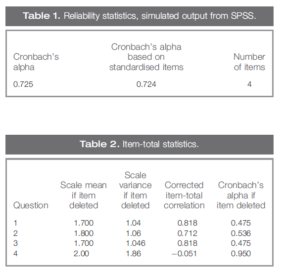
표 1은 4개의 질문에 대한 크론바흐의 알파 0.72를 보여준다. 표 2는 'Cronbach's Alpha if Item deleted'라는 제목의 열이 있는 항목-총 상관 통계를 보여줍니다. (항목-총 상관관계는 개별 질문 점수와 총 점수 사이의 상관 관계입니다.)
Table 1 shows Cronbach's alpha for four questions, 0.72. Table 2 shows item-total correlation statistics with the column headed ‘Cronbach's Alpha if Item deleted’. (Item-total correlation is the correlation between an individual question score and the total score).
시험의 네 번째 문항은 총 항목 상관 관계가 -0.51로, 이 특정 문항에 대한 응답이 총점과 음의 상관 관계를 가지고 있음을 의미합니다. 이 문제를 시험에서 제거하면 나머지 세 문제 중 알파가 0.725에서 0.950으로 증가하여 시험을 훨씬 더 신뢰할 수 있습니다.
The fourth question in the test has a total-item correlation of −0.51 implying that responses to this particular question have a negative correlation with the total score. If we remove this question from the test, the alpha of the three remaining questions increase from 0.725 to 0.950, making the test significantly more reliable.
표 3과 4는 질문 4를 제거한 후의 출력 SPSS를 보여줍니다.
Tables 3 and 4 show the output SPSS after removing Question 4:
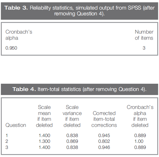
표 3과 표 4는 문제 4를 시험에서 제거하면 알파 값이 크게 증가하는 영향을 보여줍니다.
Tables 3 and 4 illustrate the impact of removing Question 4 from the test, which significantly increases the value of alpha.
그러나 이제 문제 2를 제거하면 시험에 대한 알파 값이 완벽해집니다. 즉, 1은 시험의 각 문제가 정확히 동일한 것을 측정해야 한다는 것을 의미합니다. 여러 문항이 동일한 구성을 측정하는 등 시험에 중복성이 있음을 시사하기 때문에 반드시 좋은 것은 아니다. 이 경우 신뢰성을 훼손하지 않고 테스트 길이를 단축할 수 있습니다. 신뢰성은 검정 길이의 함수이기 때문입니다. 항목이 많을수록 검정의 신뢰성이 높아집니다.
However, if we now remove Question 2, the value of the alpha for the test will be perfect, i.e. 1, which means each question in the test must be measuring exactly the same thing. This is not necessarily a good thing as it suggests that there is redundancy in the test, with multiple questions measuring the same construct. If this is the case, the test length could be shortened without compromising the reliability (Nunnally & Bernstein ). This is because the reliability is a function of test length. The more the items, the more the reliability of a test.
Cronbach의 알파와 KR-20은 검정의 신뢰성을 추정하는 데 유용하지만, [측정 오차의 모든 원인을 하나의 값으로 통합]합니다(Mushquash & O'Connor). 실제 점수는 관찰된 점수와 [다양한 출처에서 파생된 오류]를 더한 것과 동일하다는 점을 기억하십시오. 각 오차원의 영향은 일반성 계수로 추정할 수 있으며, 이는 실제 점수 모델의 신뢰도 추정치와 유사하다. 나중에 우리는 알려진 대로 일반화 가능성 이론 또는 G 이론을 사용하여 측정 오류의 원인을 식별하고 줄이는 방법을 설명할 것이다. 또한 이전 가이드에서는 문항 난이도, 문항 변별도 및 포인트 바이시리얼 계수를 CTT의 관점에서 설명하고 해석하였다.
Although Cronbach's alpha and KR-20 are useful for estimating the reliability of a test, they conflate all sources of measurement error into one value (Mushquash & O'Connor ). Recall that true scores equal observed scores plus errors, which is derived from a variety of sources. The influence of each source of error can be estimated by the coefficient of generalisability, which is similar to a reliability estimate in the true score model (Cohen & Swerdlik ). Later we will describe how to identify and reduce sources of measurement errors using generalisability theory or G-theory as it is known. What is more, in our previous Guide (Tavakol & Dennick 2012), we explained and interpreted item difficulty level, item discrimination index and point bi-serial coefficient in terms of CTT.
본 가이드에서는 이러한 개념을 항목 특성 매개 변수(항목 난이도 및 항목 변별력)를 이용한 IRT(Item Response Theory)와 래쉬 모델을 이용한 모든 질문에 대한 학생 능력/성과의 관점에서 설명하고 해석할 것이다.
In this Guide, we will explain and interpret these concepts in terms of Item Response Theory (IRT) using item characteristic parameters (item difficulty and item discrimination) and the student ability/performance to all questions using the Rasch model.
인자분석
Factor analysis
[선형 요인 분석]은 시험 개발자가 문제 수를 줄이고 중요한 문제가 시험에 포함되도록 하기 위해 널리 사용된다. 예를 들어, 심장병학 강좌 소집자는 심장병학을 가르치는 데 관련된 모든 의학 교사들에게 시험을 위한 10개의 문제를 제공하도록 요청할 수 있다. 이 경우 100개의 질문이 생성될 수 있지만, 이 모든 질문은 동일한 개념 집합을 테스트하는 것은 아닙니다. 따라서 문제들 간의 상관관계 패턴을 파악하면 시험의 기본 요소를 대상으로 하는 관련 문제를 발견할 수 있다. 요인은 일련의 질문 사이의 관계를 나타내는 구인이며, 질문이 요인과 상관관계가 있을 경우 생성됩니다. 요인 분석 언어에서, 이는 요인 '적재loadings'를 의미한다. 요인 분석이 수행된 후, 관련된 질문은 특정 명명된 구조를 나타내는 요인에 로드됩니다. 따라서 적재량이 낮은 질문은 제거하거나 수정할 수 있습니다.
Linear factor analysis is widely used by test developers in order to reduce the number of questions and to ensure that important questions are included in the test. For example, the course convenor of cardiology may ask all medical teachers involved in teaching cardiology to provide 10 questions for the exam. This might generate 100 questions, but all these questions are not testing the same set of concepts. Therefore, identifying the pattern of correlations between the questions allows us to discover related questions that are aimed at the underlying factors of the exam. A factor is a construct which represents the relationship between a set of questions and will be generated if the questions are correlated with the factor. In factor analysis language, this refers to factor ‘loadings’. After factor analysis is carried out, related questions load onto factors which represent specific named constructs. Questions with low loadings can therefore be removed or revised.
테스트가 단일 특성을 측정하는 경우, [부하가 높은 요인 하나]만 관찰된 질문 관계를 설명하므로 테스트는 단일 차원입니다. 여러 요인이 확인되면 검정은 다차원적인 것으로 간주됩니다.
If a test measures a single trait, only one factor with high loadings will explain the observed question relationships and hence the test is uni-dimensional. If multiple factors are identified, then the test is considered to be multi-dimensional.
[선형 요인 분석]에는 [탐색적 요인]과 [확인적 요인]의 두 가지 주요 요소가 있습니다.
- 탐색적 요인 분석(EFA)은 검정 내의 기본 구성 요소를 식별하고 이들 사이의 모형 관계를 가정합니다.
- 확인적 요인 분석(CFA)은 모형이 새 데이터 집합을 사용하여 데이터에 적합한지 여부를 검증합니다. 아래에서는 각 방법에 대해 설명합니다.
There are two main components to linear factor analysis: exploratory and confirmatory.
- Exploratory Factor Analysis (EFA) identifies the underlying constructs or factors within a test and hypothesises a model relationship between them.
- Confirmatory Factor Analysis (CFA) validates whether the model fits the data using a new data set. Below, each method is explained.
탐색적 요인 분석
Exploratory factor analysis
EFA는 앞에서 설명한 바와 같이 문제 간의 관계를 식별하고, 테스트에서 주요 요소를 발견하는 데 널리 사용된다. 시험 문제를 수정하거나 특정 지식 영역의 문제를 선택하는 데 사용할 수 있습니다. 예를 들어, 심장학 검사에서 관상동맥 심장 질환의 임상 징후를 검사하는 데 관심이 있는 경우, 이 영역에 로드load되는 질문을 단순히 찾습니다. 다음 시뮬레이션 예제는 50명의 학생이 10개의 문제를 출제하는 시험을 사용하여 시험에서 문제를 개선하는 방법을 보여줍니다. 이를 통해 시험 문제를 수정하고 강화하는 방법을 시연하고 관심 영역에 대한 loadings를 계산할 수 있다. EFA는 요인 식별뿐만 아니라 각 질문에 대한 '커뮤널리티communality'도 계산합니다. communality의 개념을 이해하기 위해서는 EFA 접근법 내의 분산variance(점수의 변동성)을 설명할 필요가 있다.
EFA is widely used to identify the relationships between questions and to discover the main factors in a test as previously described. It can be used either for revising exam questions or choosing questions for a specific knowledge domain. For example, if in the cardiology exam we are interested in testing the clinical manifestations of coronary heart disease, we simply look for the questions which load on to this domain. The following simulated example, using an examination with 10 questions taken by 50 students, demonstrates how to improve the questions in an examination. This allows us to demonstrate how to revise and strengthen exam questions and to calculate the loadings on the domain of interest. As well as identifying the factors EFA also calculates the ‘communality’ for each question. To understand the concept of communality, it is necessary to explain the variance (the variability in scores) within the EFA approach.
우리는 이미 기술 통계로부터 변수의 분산을 계산하는 방법을 배웠다. 요인 분석 언어에서 각 질문의 분산은 두 부분으로 구성됩니다. 한 부분은 'common variance'이라고 하는 다른 질문과 공유할 수 있는 것이 있고, 나머지는 '오류' 또는 '랜덤 분산'이라고 하는 다른 질문과 공유할 수 없습니다. 문항에 대한 communality은 특정 요인 집합으로 설명되는 분산의 값으로, 범위는 0에서 1.00 사이입니다. 예를 들어 랜덤 분산이 없는 문항은 1.00의 공통성을 가지며, 다른 문항과 분산이 공유되지 않은 문항은 0.00의 공통성을 가집니다. 문항 9(표 5)에 대한 communality은 0.85로, 즉 질문 9의 분산의 85%가 요인 1과 요인 2로 설명되며, 질문 9의 분산의 15%는 다른 문항과는 공통점이 없습니다.
We have already learnt from descriptive statistics how to calculate the variance of a variable. In the language of factor analysis, the variance of each question consists of two parts. One part can be shared with the other questions, called ‘common variance’; the rest may not be shared with other questions, called ‘error’ or ‘random variance’. The communality for a question is the value of the variance accounted for by the particular set of factors, ranging from 0 to 1.00. For example, a question that has no random variance would have a communality of 1.00; a question that has not shared its variance with other questions would have a communality of 0.00. The communality shown for Question 9 (Table 5) is 0.85, that is 85% of the variance in Question 9 is explained by factor 1 and factor 2, and 15% of the variance of Question 9 has nothing in common with any other question.
SPSS의 각 질문에 대한 공유 분산을 계산하기 위해 SPSS(SPSS)에서 다음 단계를 수행합니다. 메뉴에서 'Analyse', 'Dimension Reduction' 및 'Factor'를 각각 선택합니다. 그런 다음 모든 질문을 '변수' 상자로 이동합니다. 설명'을 선택한 다음 '초기 솔루션'과 '계수'를 각각 클릭합니다. 그런 다음 '회전'을 클릭합니다. 'Varimax'를 선택하고 'Continue'를 클릭한 다음 'OK'를 클릭합니다. 표 5에서, 우리는 SPSS 출력의 시뮬레이션 데이터를 함께 결합했다.
To compute the shared variances for each question in SPSS, the following steps are carried out in SPSS (SPSS ). From the menus, choose ‘Analyse’, ‘Dimension Reduction’ and ‘Factor’, respectively. Then move all questions on to the ‘Variables’ box. Choose ‘Descriptive’ and then click ‘Initial Solution’ and ‘Coefficients’, respectively. Then click ‘Rotation’. Choose ‘Varimax’ and click on ‘Continue’ and then ‘OK’. In Table 5, we have combined the simulated data of the SPSS output together.

표 5는 [두 가지 요인]이 나타났음을 보여줍니다. 요인 1은 질문 9, 2, 6, 10, 4, 1, 3에서 우수한 하중을 나타내고 요인 2는 질문 7, 8에서 우수한 하중을 나타내므로 이러한 항목이 요인 1, 2와 강한 상관 관계가 있음을 알 수 있습니다. 0.71보다 큰 값을 가진 하중은 우수한 것으로 간주된다는 점에 유의해야 한다(0.71 × 0.71 = 0.50 × 100. 즉, 항목과 요인 간의 공통 분산 또는 항목 내 변동의 50%를 요인의 변동으로 설명할 수 있으며, 또는 변동의 50%를 항목과 요인에 의해 설명될 수 있다), 0.63(40% 공통 변동)은 매우 양호하며, 0.45(20% 공통 분산)는 적당합니다. 0.32(공통 분산 10%)보다 작은 값은 불량으로 간주되고 전체 검정에 덜 기여하므로 이러한 값을 조사해야 합니다.
Table 5 shows that two factors have emerged. Factor 1 demonstrates excellent loading with Questions 9, 2, 6, 10, 4, 1 and 3 and Factor 2 demonstrates excellent loading with Questions 7 and 8, indicating these items have a strong correlation with Factors 1 and 2.
- It should be noted that loadings with values greater than 0.71 are considered excellent (0.71 × 0.71 = 0.50 × 100; i.e. 50% common variance between the item and the factor, or 50% of the variation in the item can be explained by the variation in the factor, or 50% of the variance is accounted for by the item and the factor),
- 0.63 (40% common variance) very good,
- 0.45 (20% common variance) fair.
- Values less than 0.32 (10% common variance) are considered poor and less contribute to the overall test and they should be investigated (Comrey & Lee ; Tabachnick & Fidell ).
표 5는 또한 h2로 표시된 열의 각 질문에 대한 communalities 을 보여준다. 예를 들어, 질문 2의 분산의 92%는 EFA 접근법에서 나타난 두 가지 요인에 의해 설명된다. 가장 낮은 communalities 은 질문 5에 대한 것이며, 분산의 8%를 기소하는 것은 이 질문으로 설명된다. 30% 미만의 낮은 값은 문제의 분산이 식별된 요인에 로드된 다른 질문과 관련이 없음을 나타냅니다. 표 5에서 질문 5는 커뮤니티 수치가 가장 낮고 요인 1 또는 2에 로드되지 않았으므로 이 질문을 수정하거나 폐기해야 합니다.
Table 5 also shows communalities for each question in the column labelled h2. For example, 92% of the variance in Question 2 is explained by the two factors that have emerged from the EFA approach. The lowest communality is for Question 5, indicting 8% of the variance is explained by this question. Low values of less than 30% indicate that the variance of the question does not relate to other questions loaded on to the identified factors. In Table 5, Question 5 has the lowest communality figure and has not loaded onto Factors 1 or 2, suggesting this question should be revised or discarded.
표 5는 또한 EFA 접근법에서 확인된 [두 가지 요인에 의해 설명되는 분산 값]을 보여줍니다. 분산의 0.47은 인자 1로, 분산의 0.23은 인자 2로 설명됩니다. 따라서 분산의 0.70은 모든 질문에 의해 설명됩니다. 그러나 질문 5를 삭제하면 총 분산이 0.78로 증가할 수 있습니다. 표 5에 대한 추가 해석은, 대다수의 문제가 인자 1에 실려서 시험의 구인 타당도에 대한 수렴 및 변별의 증거를 제공한다는 것이다.
- 인자 1에 대한 부하가 높기 때문에 테스트가 [수렴]된다고 주장할 수 있습니다.
- 또한 요인 1에 적재된 문제가 요인 2에 적재되지 않았으므로 시험은 [변별]됩니다.
즉, 요인 2는 요인 1과 구별되는 또 다른 구성/개념을 측정합니다. 두 개의 인자가 확인되었으므로 두 개의 서로 다른 구조를 측정하기 때문에 각 인자에 대한 Cronbach의 알파 계수를 계산하는 것이 적절할 것입니다. 세 가지 이상의 요인에 적재되는 문항은 조사가 필요하다는 점에 유의해야 한다.
Table 5 also shows the values of variance explained by the two factors that have been identified from the EFA approach; 0.47 of the variance is accounted for by Factor 1 and 0.23 of the variance is accounted for by Factor 2. Therefore, 0.70 of the variance is accounted for by all of the questions. However, if we delete Question 5, we can increase the total variance accounted for to 0.78. A further interpretation of Table 5 is that the vast majority of questions have been loaded on to Factor 1, providing evidence of convergence and discrimination for the construct validity of the test.
- We can argue that the test is convergent as there are high loadings on to Factor 1.
- The test is also discriminant as the questions that have loaded on to Factor 1 have not loaded on to Factor 2.
This means that Factor 2 measures another construct/concept which is discriminated from Factor 1. Because two factors have been identified, it would be appropriate to calculate Cronbach's alpha co-efficient for each factor because they are measuring two different constructs. It should be noted that items which load on more than two factors need to be investigated.
확인적 요인 분석
Confirmatory factor analysis
CFA의 기술은 심리 검사를 검증하는 데 널리 사용되었지만 시험 문제의 심리학적 특성을 평가하고 개선하는 데는 덜 사용되었다. EFA 접근 방식은 시험 문제가 어떻게 연관되거나 기저 요인 영역과 연결되는지 밝힐 수 있다. 예를 들어, EFA 접근 방식은 100문항 시험의 내부 구조가 신체 검사, 임상 추론 및 의사소통 기술 등 [세 가지 기저 영역]으로 구성되어 있음을 보여줄 수 있다. 식별된 요인의 수는 가설 모형, 즉 요인 구조 모형의 성분을 구성합니다. 위의 예제에서 모형을 3-요인 모형이라고 합니다. CFA 접근법은 잠재(기본) 요인을 확인하기 위해 [EFA에 의해 추출된 가설 모델]을 사용한다. 그러나 모형 적합을 확인하려면 순환 논리circular argument를 피하기 위해 [새 데이터 세트]를 사용해야 합니다. 예를 들어, 같은 시험을 다른 학생 그룹이나 비교 가능한 학생 그룹에 적용할 수 있다.
The technique of CFA has been widely used to validate psychological tests but has been less used to evaluate and improve the psychometric properties of exam questions. The EFA approach can reveal how exam questions are correlated or connected to an underlying domain of factors. For example, an EFA approach may show that the internal structure of a 100 question test consist of three underlying domains, say physical examination, clinical reasoning and communication skills. The number of factors identified constitutes the components of a hypothesised model, the factor structure model. In the above example, the model would be termed a three-factor model. The CFA approach uses the hypothesised model extracted by EFA to confirm the latent (underlying) factors. However, in order to confirm model fitting, a new data set must be used to avoid a circular argument. For example, the same test could be administered to a different but comparable group of students.
따라서 교육자는 먼저 EFA를 사용하여 모델을 식별하고 CFA를 사용하여 테스트해야 합니다. 또한 이 접근 방식을 통해 교육자는 시험 문제와 구성 요소(Floys & Widman)를 수정할 수 있습니다. 예를 들어, EFA가 병력 시험과 신체 검사 문제로 구성된 시험에서 2-요인 모델을 공개했다고 가정합시다. 연구자는 문제의 심리학적 특성을 측정하고 모형의 전반적인 적합성을 검정하여 시험의 타당성과 신뢰성을 향상시키려 합니다. 이것은 가설 모델에 새로 입력된 샘플 데이터의 적합도를 결정하는 구조 방정식 모델링(SEM)을 사용하여 달성될 수 있다. [모형 적합성model fit]은 카이-제곱 검정 및 기타 적합 지수를 사용하여 평가됩니다. 다른 통계 가설 검정 절차와 달리 카이-제곱 값이 [유의하지 않으면], 새 데이터가 적합하고, 모형이 확인된 것이다. 그러나 카이-제곱의 값은 표본 크기를 늘거나 줄어드는 것에 달라지는 함수이므로 [다른 적합 지수]들도 조사해야 합니다. 이러한 지수는 비교 적합 지수(CFI)와 근삿값 평균 제곱 오차(RMSEA)입니다.
- CFI 값이 0.90보다 크면 검사 데이터에 대해 심리적으로 허용 가능한 적합도를 나타냅니다.
- RMSEA 값이 0.05보다 작아야 적합성이 양호합니다. RMSEA가 0이면 모형 적합이 완벽하다는 것을 나타냅니다.
- CFA는 SAS, LISREL, AMOS 및 Mplus와 같은 다수의 인기 있는 통계 소프트웨어 프로그램에 의해 실행될 수 있다는 점에 유의해야 한다.
Therefore, educators must first identify a model using EFA and test it using CFA. This approach also allows educators to revise exam questions and the factors underlying their constructs (Floys & Widaman ). For example, suppose EFA has revealed a two-factor model from an exam consisting of history-taking and physical examination questions. The researcher wishes to measure the psychometric characteristics of the questions and test the overall fit of the model to improve the validity and reliability of the exam. This can be achieved by the use of structural equation modelling (SEM) which determines the goodness-of-fit of the newly input sample data to the hypothesised model. The model fit is assessed using Chi-square testing and other fit indices. In contrast to other statistical hypothesis testing procedures, if the value of Chi-square is not significant, the new data fit and the model is confirmed. However, as the value of Chi-square is a function of increasing or decreasing sample size, other fit indices should also be investigated (Dimitrov ). These indices are the comparative fit index (CFI) and the root mean square error of approximation (RMSEA).
- A CFI value of greater than 0.90 shows a psychometrically acceptable fit to the exam data.
- The value of RMSEA needs to be below 0.05 to show a good fit (Tabachnick & Fidell ). A RMSEA of zero indicates that the model fit is perfect.
- It should be noted that CFA can be run by a number of popular statistical software programmes such as SAS, LISREL, AMOS and Mplus.
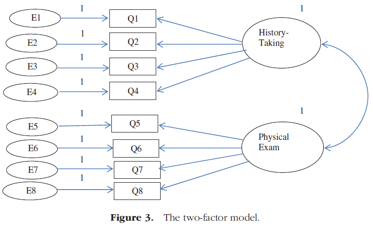
이 논문의 목적을 위해, 우리는 그것의 용이한 사용을 위해 AMOS(모멘트 구조의 분석)를 선택한다. AMOS 소프트웨어 프로그램은 모형을 쉽게 만들고 카이-제곱 값과 적합 지수를 계산할 수 있습니다. 위의 예에서, 8문항의 시험은 역사 시험과 신체 검사라는 두 가지 요소를 가지고 있으며, 이 8문항의 분산은 이 두 가지 높은 상관관계 요인에 의해 설명될 수 있다. 테스트 개발자는 AMOS에서 2-요인 모델(경로 다이어그램)을 그려 모델을 테스트합니다(그림 3). 모델의 매개변수를 추정하기 전에 '보기'를 클릭하고 '분석 특성'을 클릭한 다음 '최소화 기록', 표준화 추정치, '다중 상관 제곱' 및 '수정 지수'를 클릭합니다. 견적을 실행하려면 맨 위의 메뉴에서 '분석'을 클릭한 다음 '견적 계산'을 클릭합니다.
For the purpose of this article, we choose AMOS (Analysis of Moment Structures) for its use of ease. The AMOS software program can easily create models and calculate the value of Chi-square as well as the fit indices. In the above example, a test of 8 questions has two factors, history-taking and physical examination and the variance of these eight exam questions can be explained by these two highly correlated factors. The test developer draws the two-factor model (the path diagram) in AMOS to test the model (Figure 3). Before estimating the parameters of the model, click on the ‘view’ and click on ‘Analysis Properties’ and then click on ‘Minimization history’, Standardised estimates, ‘Squared multiple Correlations’ and ‘Modification indices’. To run the estimation, from the menu at the top, click on ‘Analyze’, then click on ‘Calculate Estimates’.
출력은 표 6에 나와 있습니다. SEM은 질문과 요인 간의 계산된 상관 관계의 기울기와 절편을 계산합니다. CTT와 비교하자면,
- 절편은 항목 난이도 지수와 유사하며
- 기울기(표준화된 회귀 가중치/계수)는 변별도와 유사합니다.
The output is given in Table 6. SEM calculates the slopes and intercepts of calculated correlations between questions and factors. From a CTT,
- the intercept is analogous to the item difficulty index and
- the slope (standardised regression weights/coefficients) is analogous to the discrimination index.

표 6은 병력탐구 1번 문항이 쉬웠고, 신체검사에서 3번 문항이 어려웠다는 것을 알 수 있다. 표 6은 또한 병력 시험 문제 4가 전체 병력시험 점수에 기여하지 않는다는 것을 보여준다. 검사 데이터에 대한 적합 모형의 정도를 평가하기 위해 추가 분석이 수행되었습니다.
Table 6 shows that Question 1 in history-taking and Question 3 in physical examination were easy (intercept = 0.97) and hard (0.08), respectively. Table 6 also shows that Question 4 in history-taking is not contributing to overall history-taking score (slope = −0.03). Further analysis was conducted to assess degree of fit model to the exam data.
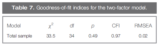
표 7에 초점을 맞추면 카이-제곱 값에 대한 유의성 결여(p = 0.49)는 새 표본에서 2-요인 모형에 대한 지지를 의미합니다. 표 7의 CFI 및 RMSEA 값을 모두 검토하면 2-요인 모형이 새 표본에 대한 검사 데이터에 가장 적합하다는 것이 명백합니다.
Focusing on Table 7, the absence of significance for the Chi-square value (p = 0.49) implies support for the two- factor model in the new sample. In reviewing values of both CFI and RMSEA in Table 7, it is evident that the two-factor model represents a best fit to the exam data for the new sample.
검사의 병력 청취 성분과 신체 검사 성분 사이의 관계에 대한 추가 증거는 가정된 2-요인 모델을 뒷받침하는 두 요인 간의 0.70 상관관계를 계산함으로써 드러난다. AMOS는 '출력 다이어그램 보기' 버튼을 클릭하여 요인/구성 요소 간의 상관 관계를 표시합니다. 또한 '텍스트 출력'에서 상관 관계 추정치를 볼 수 있습니다. 메인 메뉴에서 보기를 선택한 다음 '텍스트 출력'을 클릭합니다.
Further evidence for the relationship between the history-taking and physical examination components of the test is revealed by the calculation of a 0.70 correlation between the two factors, supporting the hypothesised two-factor model. It should be noted that AMOS will display the correlation between factors/components by clicking the ‘view the output diagram’ button. You can also view correlation estimates from ‘text output’. From the main menu, choose view and then click on ‘text output’.
일반화 가능성 이론 분석
Generalisability theory analysis
[신뢰성]은 학생들의 지식과 역량을 일관되게 측정하는 [테스트의 능력]과 관련이 있다는 점을 기억하시기 바랍니다. 예를 들어, 같은 항목과 같은 조건을 가진 학생들이 다른 경우에 같은 시험을 다시 본다면, 결과는 거의 같아야 한다. CTT에서 항목 및 조건은 획득된 점수와 관련된 측정 오류의 원인일 수 있습니다. KR-20 또는 크론바흐의 알파와 같은 신뢰성 추정치는 이러한 문항과 조건(시험의 측면facet이라고도 함)과 관련된 측정 오류의 잠재적 원인을 식별할 수 없으며, 각각을 구별할 수 없다.
We would ask you to recall that reliability is concerned with the ability of a test to measure students' knowledge and competencies consistently. For example, if students are re-examined with the same items and with the same conditions on different occasions, the results should be more or less the same. In CTT, the items and conditions may be the causes of measurement errors associated with the obtained scores. Reliability estimates, such as KR-20 or Cronbach's alpha, cannot identify the potential sources of measurement error associated with these items and conditions (also known as facets of the test) and cannot discriminate between each one.
그러나 Lee J. Cronbach와 동료들이 개발한 일반화가능도 이론 또는 G-이론이라고 불리는 CTT의 확장은 테스트 생성자가 실제 점수를 해석하기 위한 측정 오류의 원천에 대한 더 명확한 그림을 얻을 수 있도록 이러한 측면을 인식, 추정 및 분리하려고 시도한다. 예를 들어, G이론을 사용하여 OSCE 검사 결과에 대한 단일 분석으로 모든 측면을 추정할 수 있으며, 잠재적으로 시험에서 오류를 발생시킬 수 있다. 측정 오차의 각 면에는 아래에 설명된 분산 분석(ANOVA) 절차를 통해 계산되는 분산 성분variance component이라는 값이 있습니다. 이러한 분산 성분variance component은 다음으로 시험의 신뢰성과 같으며 모든 측면에 걸쳐 학생들의 평균 점수를 일반화할 수 있는 G 계수를 계산하는 데 사용됩니다.
However, an extension of CTT called Generalisability Theory or G-theory, developed by Lee J. Cronbach and colleagues (Cronbach et al. ), attempts to recognise, estimate and isolate these facets allowing test constructors to gain a clearer picture of sources of measurement error for interpreting the true score. One single analysis of, for example, the results of an OSCE examination, using G-theory can estimate all the facets, potentially producing error in the test. Each facet of measurement error has a value associated with it called its variance component, calculated via an analysis of variance (ANOVA) procedure, described below. These variance components are next used to calculate a G-coefficient which is equivalent to the reliability of the test and also enables one to generalise students’ average score over all facets.
예를 들어 OSCE가 SP, 다양한 검사자 및 다양한 항목을 사용하여 12개 스테이션에서 학생들의 성과를 평가했다고 가정해 보십시오. [평가의 한 측면]으로서 SP, 심사관 및 항목과 이들의 상호작용(예: SP와 항목 간의 상호작용)이 고려할 수 있다. 학생이 OSCE에서 얻은 점수는 이러한 [측정 오류의 측면]에 영향을 받기 때문에 평가자는 각 측면에 의해 야기되는 오류의 양을 추정해야 한다. 또한, 우리는 학생들이 시험을 이용하여 그들의 시험 수행에 대한 최종 결정을 내리는 것을 조사한다. 이 결정을 내리기 위해서, 우리는 그 점수에 근거하여 각 학생에 대한 시험 점수를 일반화할 필요가 있다. 이것은 평가자들이 좋은 결정을 내리기 위한 수단으로서 점수의 신뢰성과 신뢰성을 보장해야 한다는 것을 나타낸다. 따라서 테스트에서 얻은 관측(취득) 점수와 관련된 오류의 구성을 조사할 필요가 있다. 그런 다음 G-이론 분석은 확인된 오류의 원인을 최소화하기 위해 테스트 생성자에게 유용한 정보를 제공할 수 있다. 이제 분산 성분에서 G-계수를 계산하는 방법을 설명하겠습니다.
For example, imagine an OSCE has used SPs, a range of examiners and various items to assess students' performance on 12 stations. SPs, examiners and items and their interactions (e.g. interaction between SPs and items) are considered as facets of the assessment. The score that the student obtains from the OSCE will be affected by these facets of measurement error and therefore the assessor should estimate the amount of error caused by each facet. Furthermore, we examine students using a test to make a final decision regarding their performance on the test. To make this decision, we need to generalise a test score for each student based on that score. This indicates that assessors should ensure the credibility and trustworthy of the score as means to making a good decision (Raykov & Marcoulides ). Therefore, the composition of errors associated with the observed (obtained) scores that gained from a test need to be investigated. G-theory analysis can then provide useful information for test constructors to minimise identified sources of error (Brennan ). We will now explain how to calculate the G-coefficient from variance components.
G-계수 계산
G-coefficient calculation
Facet의 분산 성분에서 G-계수를 계산하기 위해 검정 분석가는 전통적으로 ANOVA 절차를 사용합니다. ANOVA은 검사에 존재하는 [총 분산]을 측정 오차의 원인인 [두 개 이상의 성분]으로 분할하는 통계적 절차입니다. 조사자는 분산 분석 결과(예: SP, 항목, 평가자 등)에서 각 변동 소스의 계산된 평균 제곱을 사용하여 분산 성분을 결정한 다음 이러한 값에서 G-계수를 계산합니다.
To calculate the G-coefficient from variance components of facets, test analysers traditionally use the ANOVA procedure. ANOVA is a statistical procedure by which the total variance present in a test is partitioned into two or more components which are sources of measurement error. Using the calculated mean square of each source of variation from the ANOVA output (e.g. SPs, items, assessors, etc.), investigators determine the variance components and then calculate the G-coefficient from these values.
그러나 SPSS 및 통계 분석 시스템(SAS)과 같은 기타 통계 패키지를 통해 이제 테스트 데이터에서 직접 분산 성분을 계산할 수 있습니다. 이제 G-계수를 계산하기 위해 SPSS에서 직접 분산 성분을 얻는 방법을 설명하겠습니다. 사용되는 절차는 테스트의 facet 수에 따라 달라집니다. 아래 설명된 바와 같이 단일 패싯 및 다중 패싯 설계가 있습니다.
However, SPSS and other statistical packages like the Statistical Analysis System (SAS) now allow us to calculate the variance components directly from the test data. We will now illustrate how to obtain the variance components from SPSS directly for calculating the G-coefficient. The procedure used varies according to the number of facets in the test. There are single facet and multiple facet designs as described below.
단면 설계
Single facet design
[단일 facet 설계]는 테스트에서 측정 오류의 단일 소스만 검사하지만 실제로는 다른 요소가 존재할 수 있습니다. 예를 들어, OSCE 시험에서 오류의 원인으로서 검사자의 영향에 초점을 맞추고자 할 수 있다. G이론에서, 이를 일면 '학생(들)과 시험자(e)가 교차하는' 설계라고 한다: (s × e). 3명의 검사관이 5개 항목의 1-5 체크 리스트를 사용하여 3개의 서로 다른 스테이션에서 임상 학생의 코호트를 독립적으로 평가하는 OSCE를 고려해보자. 따라서 총 점수 범위는 5에서 25까지이며, 더 높은 표시는 각 스테이션에서 더 높은 수준의 성능을 나타냅니다. G이론을 이용하여 검사자들이 어느 정도의 측정 오차를 발생시키는지 알 수 있다. 그림 4의 SPSS 데이터 편집기에는 설명 목적으로 10명의 학생과 3명의 시험관만이 제시되어 있다.
A single facet design examines only a single source of measurement error in a test although in reality others may exist. For example, in an OSCE examination, we might like to focus on the influence of examiners as sources of error. In G-theory, this is called a one-facet ‘student (s) crossed-with-examiner (e)’ design: (s × e). Consider an OSCE in which three examiners independently rate a cohort of clinical students on three different stations using a 1–5 check list of 5 items. The total mark can therefore range from 5 to 25, with higher mark suggesting a greater level of performance in each station. Using G-theory, we can find out what amount of measurement error is generated by the examiners. For illustrative purpose, only 10 students and the three examiners are presented in the Data Editor of SPSS in Figure 4.

분석하기 전에 데이터를 재구성해야 합니다. 이를 위해 화면 상단의 데이터 메뉴에서 '구조조정'을 클릭하고 해당 지침을 따른다. 그림 5에는 재구성된 데이터 형식이 나와 있습니다.
Before analysing, the data needs to be restructured. To this end, from the data menu at the top of the screen, one clicks on ‘restructure’ and follows the appropriate instructions. In Figure 5, the restructured data format is presented.

[분산 성분]을 얻기 위해 다음 단계를 수행합니다.
To obtain the variance components, the following steps are carried out:
메뉴에서 '분석'과 '일반 선형 모형'을 각각 선택합니다. 그런 다음 '분산 구성 요소'를 클릭합니다. '점수'를 클릭한 다음 화살표를 클릭하여 '종속 변수'로 표시된 상자로 '점수'를 이동합니다. 학생과 시험관을 클릭하여 '임의 요인'으로 이동합니다. '분산 추정치'가 나타나면 확인을 클릭하면 결과에 대한 각 분산 소스의 기여도가 표 8과 같이 표시됩니다.
From the menus chooses ‘Analyse’, ‘General Linear Model’, respectively. Then click on ‘variance components’. Click on ‘Score’ and then click on the arrow to move ‘Score’ into the box marked ‘dependent variable’. Click on student and examiner to move them into ‘random factors’. After ‘variance estimates’ appears, click OK and the contribution of each source of variance to the result is presented as shown in Table 8.

표 8은 학생과 검사자와 관련된 추정 분산 성분이 각각 10.144와 1.578임을 보여줍니다. 전체 분산의 백분율로 표현하면 40.00%는 학생, 6.20%는 평가자에 의한 것임을 알 수 있다. 그러나 [학생들의 분산]은 학생 코호트 내에서 이러한 변동이 예상되기 때문에 측정 오차의 한 측면으로 간주되지 않으며, G이론 측면에서는 '측정 대상'(Mushquash & O'Connor)으로 불린다. 우리의 분석에 중요한 것은, 조사자들이 전체 변동성의 6.20%를 생성했다는 것을 나타내며, 이는 상당히 낮은 값으로 간주된다. 값이 높을수록 검사자가 시험에 미치는 영향에 대한 우려가 생깁니다. 잔차 분산은 특정 원인에 기인하지 않는 분산의 양이지만 서로 다른 면과 검정 측정 대상 사이의 교호작용과 관련이 있습니다. 이 예제에서는 분산의 53.80%인 13.656을 이 인자로 설명합니다.
Table 8 shows that the estimated variance components associated with student and examiner are 10.144 and 1.578, respectively. Expressed as a percentage of the total variance, it can be seen that 40.00 % is due to the students and 6.20 % to the examiners. However, the variance of the students is not considered a facet of measurement error as this variation is expected within the student cohort and in terms of G-theory, it is called the ‘object of measurement’ (Mushquash & O'Connor ). Importantly for our analysis, the findings indicate that the examiners generated 6.20% of the total variability, which is considered a reasonably low value. Higher values would create concern about the effect of the examiners on the test. The residual variance is the amount of variance not attributed to any specific cause but is related to the interaction between the different facets and the object of measurement of the test. In this example, 13.656 or 53.80% of the variance is accounted for by this factor.
표 8의 결과를 바탕으로, 우리는 이제 일반화 계수를 계산할 수 있는 위치에 있다. 이 경우 G-계수는 [학생 분산 성분]의 비율로 정의됩니다(표시됨).
On the basis of the findings of Table 8, we are now in a position to calculate the generalisability coefficient. In this case, the G-coefficient is defined as the ratio of the student variance component (denoted

) [학생 분산 성분과 잔차 분산의 합]에 대해
) to the sum of the student variance component and the residual variance (denoted

)를 심사관 수(k)로 나누고 다음과 같이 작성한다.
) divided by the number of examiners (k) (Nunnally and Bernstein ) and written as follows:

위에서 값을 삽입하면 다음과 같은 이점이 있습니다.
Inserting the values from above, this gives:
G-계수는 전통적으로 λ 2로 표현되며, 0에서 1.0 사이의 값을 갖는 잘 알려진 신뢰도 계수의 상대이다. (위에서 설명한 단일 면 설계의 G-계수는 (비이분성 데이터의 경우) 크론바흐의 알파 계수 및 (이분성 데이터의 경우) 쿠더-리처드슨 20과 동일하다는 점에 주목할 필요가 있다.) G-계수 값의 해석은 분산 성분에서 계산된 여러 오차원을 고려하여 검정의 신뢰도를 나타낸다는 것입니다. G-계수의 값이 높을수록, 우리는 학생들의 점수에 더 많이 의존할 수 있고(일반화할 수 있음) 연구 면study facet의 영향을 덜 받았다. 위의 예제에서 G-계수는 상당히 높은 값을 가지며 검사자에 대한 분산 성분은 낮습니다. 이는 수험생들이 채점에 큰 편차가 없었음을 보여주며, 학생들의 점수에 대한 자신감을 가질 수 있음을 보여준다.
The G-coefficient, traditionally depicted as ρ 2, is the counterpart of the well-known reliability coefficient with values ranging from 0 to 1.0. (It is worth noting that the G-coefficient in the single facet design described above is equal to Cronbach's alpha coefficient (for non-dichotomous data) and to Kuder–Richardson 20 (for dichotomous data). The interpretation of the value of the G-coefficient is that it represents the reliability of the test taking into account the multiple sources of error calculated from their variance components. The higher the value of the G-coefficient, the more we can rely on (generalise) the students’ scores and the less influence the study facets have been. In the above example, the G-coefficient has a reasonably high value and the variance component for examiners is low. This shows that the examiners did not have significant variation in scoring students and that we can have confidence in the students’ scores.
다면 디자인
A multi-facet design
OSCE 시험에는 심사관 외에도 고려해야 할 [여러 가지 잠재적 facet]이 분명히 있다. 예를 들어, 스테이션 수, SP 수 및 OSCE 체크리스트의 항목 수. 이제 이전 예에서 다면 설계 건물에 대한 분산 성분과 G-계수를 계산하는 방법을 설명하겠습니다. 이제 세 개의 스테이션 각각에는 SP와 학생 개개인의 종합 점수로 이어지는 5개 문항 체크리스트가 있습니다. 여기서 [시험관, 스테이션, SP 및 문항]은 학생 성과에 영향을 미칠 수 있으므로 측정 오류의 한 단면이다.
Clearly in an OSCE examination, there are a number of other potential facets that need to be taken into consideration in addition to the examiners. For example, the number of stations, the number of SPs and the number of items on the OSCE checklist. We will now explain how to calculate the variance components and a G-coefficient for a multi-facet design building on the previous example. Each of three stations now has a SP and a 5-item checklist leading to an overall score for each student. Here, examiners, stations, SPs and items can affect the student performance and hence are facets of measurement error.
그러나 현재 오류의 원인으로 숫자 항목의 영향에 관심이 있기 때문에 각 항목(i), 각 학생(s), 각 스테이션(st), 각 SP(sp) 및 각 검사자(e)에 대한 점수를 입력해야 합니다. 검사 데이터를 SPSS에 입력하고 재구성한 후 앞서 설명한 대로 분산 성분 분석을 수행합니다. 표 9는 OCSE 결과의 잠재적 측정 오류 소스에 대한 분산 성분의 가상 결과를 보여줍니다.
However, because we are now interested in the influence of the number items as a source of error, we need to input the score for each item (i), for each student (s), for each station (st), for each SP (sp) and for each examiner (e). After entering exam data into SPSS and restructuring it, analysis of variance components is carried out as described before. Table 9 shows the hypothetical results of variance components for potential sources of measurement error in the OCSE results.

표 9는 측정 오류의 원인 중 59.16%, 16.37%, 15.04가 각각 학생, 항목 및 검사자 간의 상호작용, 학생과 검사자 및 검사자 간의 상호작용에 의해 발생함을 보여준다. 다른 면들의 조합들 사이의 잔차 분산이 부족하다는 것은 이러한 상호작용으로 인해 학생 점수가 변동할 수 없으며 결과적으로 측정 오차로 이어지지 않는다는 것을 나타낸다. 표 9의 검사관에 대한 분산 성분 값(0.06)은 표 8(1.57)의 값과 다릅니다. 다면 행렬을 만들 때 모든 관측소에 대한 총점보다는 학생들의 개별 항목 점수를 사용하기 때문입니다. 이러한 결과는 또한 각 시험관이 학생에게 부여한 실제 점수(2.88%)에 대해 거의 이견이 없음을 나타낸다. 표 8에 나와 있는 각 면과 관련된 수치와 분산 성분의 값을 다음 방정식에 삽입할 수 있습니다.
Table 9 shows that 59.16 %, 16.37 % and 15.04 of the sources of measurement error are generated by interactions between student, item and examiner, interactions between student and examiner and student, respectively. The lack of residual variance between other combinations of facets indicates that student scores cannot fluctuate owing to these interactions and consequently they do not lead to any measurement error. The value for the variance component for examiners (0.06) in Table 9 differs from the value in Table 8 (1.57) because in creating the multi-facet matrix, we are using individual item scores from students rather than their total mark for all stations. These findings also indicate that there is little disagreement about the actual scores given to student by each examiner (2.88%). We can insert the values of the variance components and the numbers associated with each facet shown in Table 8 into the following equation:

분산 성분의 0 값은 삽입되지 않으므로 SP 및 스테이션을 제외합니다.
Zero values of variance components are not inserted, thus excluding SPs and stations.
이 예에서 G-계수는 높고 패싯의 분산 성분은 낮으므로 OSCE의 신뢰성은 매우 우수합니다. 특정 측면에 대해 더 높은 분산 성분 값이 발견되면 더 자세히 조사해야 합니다. 이로 인해 검사관에 대한 교육이 개선되거나 검사 목록 또는 스테이션 수의 항목을 수정할 수 있습니다. 이러한 가상 데이터로 나타난 높은 G 계수를 고려할 때, 우리는 원칙적으로 G의 상당히 높은 값을 유지하면서 개별 면에 대한 k의 값을 줄일 수 있으며, 따라서 OSCE 시험의 신뢰성을 유지할 수 있다. OSCE의 현실 세계에서, 이것은 단순화와 OSCE 심사 비용의 감소로 이어질 수 있다. Cronbach의 알파 통계량은 G에 대해 허용 가능한 값에 대해 0.7에서 0.95 사이의 다양한 견해를 가지고 있다. 검사 요인들이 측정 오류의 근원에 어떻게 영향을 미칠 수 있는지 보기 위해 일반화 방정식을 조작하는 이러한 능력은 [의사결정 연구 또는 D-연구]의 핵심에 있다. 따라서 G-이론과 D-연구는 Cronbach의 알파 통계를 측정하는 것만으로 숨겨진 검사에서 발생하는 다양한 과정에 대한 더 큰 통찰력을 제공한다. 이를 통해 평가자는 훨씬 더 구체적이고 증거에 기반한 방식으로 평가의 질을 향상시킬 수 있습니다.
In this example, the G-coefficient is high and the variance components of the facets are low, hence the reliability of the OSCE is very good. If higher values of variance components are found for particular facets, then they need to be examined in more detail. This might lead to better training for examiners or modifying items in checklists or the number of stations. Given the high G-coefficient shown with these hypothetical data, we could in principle reduce the values of k for individual facets whilst maintaining a reasonably high value of G and hence maintaining the reliability of the OSCE exam. In the real world of OSCEs, this could lead to simplifications and a reduction in the cost of OSCE examining. As for Cronbach's alpha statistic, there are different views concerning acceptable values for G ranging from 0.7 to 0.95 (Tavakol and Dennick , b). This ability to manipulate the generalisability equation in order to see how examination factors can influence sources of measurement error and hence reliability lies at the heart of decision study or D-study (Raykov & Marcoulides ). Thus G-theory and D-study provide a greater insight into the various processes occurring in examinations, hidden by merely measuring Cronbach's alpha statistic. This enables assessors to improve the quality of assessments in a much more specific and evidence-based way.
IRT와 래쉬 모델링
The IRT and Rasch modelling
테스트 생성자는 전통적으로 [CTT 모델]을 사용하여 테스트 테스트의 신뢰성을 정량화했습니다. 예를 들어, 항목 분석(항목 난이도 및 항목 식별), 전통적인 신뢰도 계수(예: KR-20 또는 Cronbach의 알파), 항목-합계 상관 관계 및 요인 분석을 사용하여 검정의 신뢰성을 조사합니다. 우리는 방금 어떻게 G 이론을 사용하여 신뢰도를 모니터링하고 개선하기 위해 검사 조건을 보다 정교한 분석을 할 수 있는지 보여주었다. CTT는 시험과 그 오류에 초점을 맞추지만, [학생들의 능력]이 시험 및 문항과 어떻게 상호작용하는지에 대해서는 거의 언급하지 않는다. 한편, IRT의 목적은 문항의 질을 향상시키기 위해 [학생의 능력]과 [문항의 난이도] 사이의 관계를 측정하는 것이다. 이러한 유형의 분석은 컴퓨터 적응 테스트(CAT)를 위한 더 나은 질문 뱅크를 구축하는 데도 사용될 수 있다.
Test constructors have traditionally quantified the reliability of exam tests using the CTT model. For example, they use item analysis (item difficulty and item discrimination), traditional reliability coefficients (e.g. KR-20 or Cronbach's alpha), item-total correlations and factor analysis to examine the reliability of tests. We have just shown how G-theory can be used to make more elaborate analyses of examination conditions with a view to monitoring and improving reliability. CTT focuses on the test and its errors but says little about how student ability interacts with the test and its items (Raykov & Marcoulides ). On the other hand, the aim of IRT is to measure the relationship between the student's ability and the item's difficulty level to improve the quality of questions. Analyses of this type can also be used to build up better question banks for Computer Adaptive Testing (CAT).
해부학 시험을 치르는 학생을 생각해 보세요. 학생이 항목 1을 올바르게 답할 수 있는 확률은 학생의 해부학적 능력과 항목의 난이도에 영향을 받습니다. 학생이 해부학 지식 수준이 높으면 1번 항목에 정답을 맞출 확률이 높다. 난이도가 낮은 항목(즉, 어려운 항목)의 경우 학생이 해당 항목을 올바르게 답할 확률은 낮습니다. IRT는 학생 시험 점수와 항목 난이도, 항목 판별, 항목 공정성, 추측 및 성별 또는 학년와 같은 기타 학생 속성과 같은 요인(파라미터)을 사용하여 이러한 관계를 분석하려고 시도한다. IRT 분석에서는 위의 parameters로 학생 능력의 교정을 나타내는 항목 맵뿐만 아니라 학생 능력과 올바른 항목 응답 확률 사이의 관계를 보여주는 그래프가 생성된다. 또한 나중에 설명하는 항목 및 학생에 대한 '적합' 통계를 보여 주는 표입니다.
Consider a student taking an exam in anatomy. The probability that the student can answer item 1 correctly is affected by the student's anatomy ability and the item's difficulty level. If the student has a high level of anatomical knowledge, the probability that he/she will answer the item 1 correctly is high. If an item has a low index of difficulty (i.e. a hard item), the probability that the student will answer the item correctly is low. IRT attempts to analyse these relationships using student test scores plus factors (parameters) such as item difficulty, item discrimination, item fairness, guessing and other student attributes such as gender or year of study. In an IRT analysis, graphs are produced showing the relationship between student ability and the probability of correct item responses, as well as item maps depicting the calibrations of student abilities with the above parameters. Also tables showing ‘fit’ statistics for items and students, to be described later.
다양한 형태의 IRT가 도입되었다. [항목 난이도]와 [학생 능력] 간의 관계만을 살펴보려면 단일 모수 로지스틱 IRT(1PL)를 사용한다. 이것은 1960년대에 이것을 추진했던 덴마크의 통계학자를 기리기 위해 라쉬 모델이라고 불린다. 래쉬 모형은 [개념적 능력]과 [항목 난이도]를 고려하여 학생이 문항에 올바르게 답할 확률을 평가합니다. 문항 변별도, 문항 난이도, 성별 또는 연구 년도와 같은 추가 매개 변수가 포함될 수 있는 경우 2-모수 IRT(2PL) 또는 3-모수 IRT(3PL)도 사용할 수 있다. 이 기사의 목적을 위해, 우리는 1PL 또는 래쉬 모델링에 집중할 것이다.
A variety of forms of IRT have been introduced. If we wish to look at the relationship between item difficulty and student ability alone, we use the one-parameter logistic IRT (1PL). This is called the Rasch model in honour of the Danish statistician who promoted it in the 1960s. The Rasch model assesses the probability that a student will answer an item correctly given their conceptual ability and the item difficulty. Two-parameter IRT (2PL) or three-parameter IRT (3PL) are also available where further parameters such as item discrimination, item difficulty, gender or year of study can be included. For the purposes of this article, we are going to concentrate on 1PL or Rasch modelling.
[래쉬 모델링]에서 학생들의 능력 점수 및 항목 난이도의 값은 해석을 쉽게 하기 위해 [표준화]된다.
- 평균을 표준화하면 학생 능력 수준은 0으로, SD는 1로 설정된다.
- 마찬가지로 평균 문항 난이도는 0으로, SD는 1로 설정된다.
따라서 표준화 후 평균 점수 0점을 받은 학생은 평가 대상 항목에 대한 평균 능력을 갖게 된다. 1.5의 점수로, 학생의 능력은 평균보다 SD가 높은 1.5이다. 마찬가지로 난이도가 0인 항목은 평균 항목으로 간주되고 난이도가 2인 항목은 어려운 문항으로 간주됩니다. 일반적으로, 주어진 문항의 값이 양수이면 해당 항목은 해당 학생의 코호트에게 어렵고, 값이 음수이면 해당 문항은 쉽다.
In Rasch modelling, the scores of students’ ability and the values of item difficulty are standardised to make interpretation easier.
- After standardising the mean, student ability level is set to 0 and the SD is set to 1.
- Similarly, the mean item difficulty level is set to 0 and the SD is set to 1.
Therefore, after standardisation a student who receives a mean score of 0 has an average ability for the items being assessed. With a score of 1.5, the student's ability is 1.5, SDs above the mean. Similarly, an item with a difficulty of 0 is considered an average item and an item with a difficulty of 2 is considered to be a hard item. In general, if a value of a given item is positive, that item is difficult for that cohort of students and if the value is negative, that item is easy (Nunnally & Bernstein ).
학생 능력과 항목 난이도를 표준화하기 위해 표 10을 참고하여, 7명의 학생 해부학 시험에서 7개 항목에 대한 시뮬레이션된 이분법 데이터를 제시하여, 각 학생에 대한 학생 능력과 7개 항목의 난이도를 보여준다. θ라고 불리는, 학생의 능력을 계산하기 위해, 각 학생에 대해 부정확한 분수에 대한 올바른 분수의 비율의 자연 로그가 취해진다. 예를 들어 학생 2(θ2)의 능력은 다음과 같이 계산된다.
To standardise the student ability and item difficulty, consider Table 10, presenting the simulated dichotomous data for seven items on an anatomy test from seven students showing the student ability for each student and the difficulty level for each of the seven items. To calculate the ability of the student, which is called θ , the natural logarithm of the ratio of the fraction correct to the fraction incorrect (or 1 – fraction correct) for each student is taken. For example, the ability of student 2 (θ2) is calculated as follows:
이것은 학생 2의 능력이 평균 SD보다 0.89라는 것을 나타냅니다. b라고 불리는 각 항목의 난이도를 계산하기 위해, 각 항목에 대해 정확한 분수에 대한 잘못된 분수의 비율(또는 1 – 분수가 정확함)의 자연 로그가 계산됩니다. 예를 들어 항목 2의 난이도는 다음과 같이 계산한다.
This indicates that the ability of student 2 is 0.89 above the mean SD. To calculate the difficulty level of each item which is called b, the natural log of the ratio of the fraction incorrect (or 1 – fraction correct) to the fraction correct for each item is calculated. For example, the difficulty of item 2 is calculated as follows:

값이 -1.73이면 항목이 비교적 쉽다는 것을 나타냅니다. 이 표준화 프로세스는 모든 학생과 모든 항목에 대해 수행되며 Excel 스프레드시트(표 10)에서 쉽게 수행할 수 있습니다.
A value of −1.73 suggests that the item is relatively easy. This standardisation process is carried out for all students and all items and can easily be facilitated in an Excel spreadsheet (Table 10).

우리는 이제 [특정 능력을 가진 학생]이 [특정 항목 난이도를 가진 질문]에 정확하게 답할 확률을 추정하는 위치에 있다. 1PL의 경우 다음 방정식을 사용하여 확률을 추정합니다.
We are now in a position to estimate the probability that a student with a specific ability will correctly answer a question with a specific item difficulty. For 1PL, the following equation is used to estimate the probability:

여기서 p는 확률, θ 는 학생 능력, b는 항목 난이도입니다. 표 10을 참조하면, 학생 1의 능력은 평균 -0.28 SD 이하이며, 난이도 -1.73의 1번 문항이 정답으로 평균 이하이다. 위 공식을 기준으로 학생 1이 항목 1을 맞힐 확률은 [1/(1+e-(-0.28-(-1.73)))] = 0.12입니다. 학생 3의 능력 수준과 4번 항목의 난이도를 고려할 때, 학생이 3번 항목을 맞힐 확률은 [1/(1+e-(0.28-(0.28)] = [1/(1+e0)]입니다. = 0.50. 이는 학생 능력 수준과 항목 난이도가 일치할 경우 학생이 정답을 선택할 확률이 50%로 우연에 해당한다는 것을 보여준다.
Where p is the probability, θ is the student ability and b the item difficulty. Referring to Table 10, the ability of student 1 is −0.28 SD below the average, and item 1, with a difficulty level of −1.73, was answered correctly, which is below the average. On the basis of the above formula, the probability that student 1 will answer item 1 correctly is [1/(1 + e−(−0.28−(−1.73))] = 0.12. Considering student 3's ability level and the difficulty of item 4, the probability that the student will answer correctly item 3 is [1/(1 + e−(0.28−(0.28))] = [1/(1 + e0)] = 0.50. This shows that if the level of student ability and the level of item difficulty are matched, the probability that the student will select the correct answer is 50%, which is equal to chance.
래쉬 분석의 기본 목표는 난이도와 학생 능력에 맞는 시험 항목을 만드는 것이다. 간단히 말해서, 학생들의 '똑똑함'은 항목의 '똑똑함'과 일치해야 한다. 표 11의 자료는 학생 능력과 항목 난이도의 관계를 더 자세히 조사하기 위해 표 10에서 추출한 자료와 위의 방정식을 사용하여 학생이 항목 난이도(b)로 항목 1에 답할 확률(p)을 정확하게 제시하였다.
The fundamental aim of Rasch analysis is to create test items that match their degree of difficulty with student ability. In simple terms, the ‘cleverness’ of the students should be matched with the ‘cleverness’ of the items. In order to further examine the relationship between student ability and item difficulty, the data in Table 11 shows the probability (p) that a student will answer item 1, with item difficulty (b), correctly given their ability (θ) using data taken from Table 10 and using the equation above.

문항 특성 곡선
Item characteristic curves
Rasch 분석에서, [문항 난이도]와 [학생 능력] 사이의 관계는 그림 6에 표시된 문항 특성 곡선(ICC)으로 그래픽으로 표현된다.
In Rasch analysis, the relationship between item difficulty and student ability is depicted graphically in an item characteristic curve (ICC) shown in Figure 6.

그림 6에서는 [문항 1]의 특성을 해석하기 위해 점선을 그립니다. -1.85의 능력을 가진 학생들이 이 질문에 올바르게 답할 확률은 50%입니다. 이것은 낮은 능력을 가진 학생들이 이 질문에 정확하게 대답할 수 있는 동등한 기회를 가지고 있다는 것을 암시한다. 또한 평균 능력(수치 = 0)을 가진 학생은 정답을 말할 확률이 80%입니다. 그 의미는 이 문제가 너무 쉽다는 것이다. 세타 축을 따라 어떤 항목이 곡선을 왼쪽으로 이동시키면 쉬운 항목이 되고, 어려운 문항은 곡선을 오른쪽으로 이동시킨다는 점에 유의해야 한다. 그림 8에 표시된 검사 분석에서 추출한 항목에 대한 ICC 곡선의 예는 그림 7에 나와 있습니다. 그림 7(a)는 어려운 문제(질문 101), 그림 7(b)는 쉬운 문제(질문 3)를 보여줍니다. 그림 7(c)는 평균 능력의 학생들이 정답을 낼 확률이 50%인 '완벽한' 문제(46번 문제)를 보여준다.
In Figure 6, dotted lines are drawn to interpret the characteristics of item 1. There is a 50% probability that students with an ability of −1.85 will answer this question correctly. This implies that student with lower ability have an equal chance of answering this question correctly. In addition, a student with an average ability (θ = 0) has an 80% chance of giving a correct answer. The implication is that this question is too easy. It should be noted that if an item shifts the curve to the left along the theta axis, it will be an easy item and a hard item will shift the curve to right. Examples of ICC curves for items taken from an examination analysis shown in Figure 8 are displayed in Figure 7. Figure 7(a) shows a difficult question (Question 101) and Figure 7(b) shows an easy question (Question 3). Figure 7(c) shows the ‘perfect’ question (Question 46) in which students of average ability have a 50% chance of giving the correct answer.


항목-학생 지도
Item-student maps
학생의 능력분포와 각 항목의 난이도는 항목-학생지도(ISM)에서도 나타낼 수 있으며, Winsteps®(Linacre, )와 같은 IRT 소프트웨어 프로그램을 활용하여 항목 난이도와 학생 능력을 함께 계산하여 표시할 수 있습니다. 그림 8은 지식 기반 테스트의 데이터를 사용하는 ISM을 보여줍니다. 지도가 두 쪽으로 갈라져 있다. [왼쪽]은 학생들의 능력을 나타내며, [오른쪽]은 각 문항의 난이도를 나타낸다. 각 학생의 능력은 '해시'(#)와 '점'(.)으로 표시되며, 문항은 문항 번호로 표시됩니다.
The distribution of students’ ability and the difficulty of each item can also be presented on an Item–student map (ISM). Using IRT software programmes such as Winsteps® (Linacre, ) item difficulty and student ability can be calculated and displayed together. Figure 8 shows the ISM using data from a knowledge-based test. The map is split into two sides. The left side indicates the ability of students whereas the right side shows the difficulty of each item. The ability of each student is represented by ‘hash’ (#) and ‘dot’ (.), items are shown by their item number.
항목 난이도 및 학생 능력 값은 자연 로그를 사용하여 수학적으로 변환되며 측정 단위는 '로짓'이라고 합니다. 로짓 척도를 사용하면 값 간의 차이를 정량화할 수 있으며 척도의 동일한 거리는 동일한 크기입니다. 척도가 높을수록 항목 난이도와 학생 능력 모두 높아집니다. 'M', 'S', 'T' 문자는 각각 항목 난이도와 학생 능력의 평균, 표준 편차 1개와 표준 편차 2개를 나타냅니다. 항목 난이도의 평균이 0으로 설정되어 있습니다. 따라서, 예를 들어, 항목 46, 18, 28은 각각 0, 1, 그리고 -1의 항목 난이도를 갖는다. 로짓 능력이 0인 학생은 46, 60 또는 69번 항목에 올바르게 답할 확률이 50%입니다. 같은 학생이 항목 28과 62와 같이 덜 어려운 항목에 정확하게 답할 확률이 50% 이상이다. 또 같은 학생이 64번, 119번 등 더 어려운 항목에 정답을 맞출 확률은 50% 미만이다.
Item difficulty and student ability values are transformed mathematically, using natural logarithms, into an interval scale whose units of measurement are termed ‘logits’. With a logit scale, differences between values can be quantified and equal distances on the scale are of equal size (Bond & Fox ). Higher values on the scale imply both greater item difficulty and greater student ability. The letters of ‘M’, ‘S’ and ‘T’ represents mean, one standard deviation and two standard deviations of item difficulty and student ability, respectively. The mean of item difficulty is set to 0. Therefore, for example, items 46, 18 and 28 have an item difficulty of 0, 1, and −1 respectively. A student with an ability of 0 logits has a 50% chance of answering items 46, 60 or 69 correctly. The same student has a greater than 50% probability of correctly answering items less difficult, for example items 28 and 62. In addition, the same student has a less than 50% probability of correctly answering more difficult items such items 64 and 119.
그림 8의 ISM을 보면 이제 테스트의 속성을 해석할 수 있습니다.
- 첫째, 학생분포는 학생들의 능력이 평균보다 높은 반면, 절반 이상의 문항은 평균보다 낮은 어려움을 가지고 있다.
- 둘째, [왼쪽 상단의 학생들]은 [오른쪽 하단의 문항]보다 '똑똑'하며, 이는 문항이 쉽고 도전적이지 않았다는 것을 의미한다.
- 셋째, 대부분의 학생들은 오른쪽 상단에 잘 어울리는 항목과 왼쪽 아래에 학생이 없는 항목과 반대쪽에 위치한다. 하지만 101, 40, 86, 29번 항목은 너무 어려워서 대부분의 학생들이 할 수 있는 능력 밖이다.
By looking at the ISM in Figure 8 we can now interpret the properties of the test.
- First, the student distribution shows that the ability of students is above the average, whereas more than half of the items have difficulties below the average.
- Second, the students on the upper left side are ‘cleverer’ than the items on the lower right side meaning that the items were easy and unchallenging.
- Third, most students are located opposite items to which they are well matched on the upper right and there are no students on the lower left side. However, items 101, 40, 86 and 29 are too difficult and beyond the ability of most students.
전반적으로, 이 예에서 학생들은 대부분의 문항보다 '더 똑똑하다'. 오른쪽 아래 사분면에 있는 많은 항목은 너무 쉬우므로 검사, 수정 또는 테스트에서 삭제해야 합니다. 마찬가지로, 어떤 항목들은 분명히 너무 어렵다. 래쉬 분석의 장점은 테스트 개발자가 항목의 심리학적 특성을 개선할 수 있도록 학생 및 항목 특성을 모두 캡슐화하는 다양한 데이터 디스플레이를 생성한다는 것이다. 항목을 학생 능력에 일치시킴으로써, 우리는 항목의 진실성과 유효성을 개선하고 컴퓨터 적응 테스트의 미래에 유용한 더 높은 품질의 항목 은행을 개발할 수 있다.
Overall, in this example, the students are ‘cleverer’ than most of the items. Many items in the lower right hand quadrant are too easy and should be examined, modified or deleted from the test. Similarly, some items are clearly too difficult. The advantage of Rasch analysis is that it produces a variety of data displays encapsulating both student and item characteristics that enable test developers to improve the psychometric properties of items. By matching items to student ability, we can improve the authenticity and validity of items and develop higher quality item banks, useful for the future of computer adapted testing.
결론들
Conclusions
OSCE 스테이션뿐만 아니라 객관적인 테스트는 학생들의 숙련도를 측정하는 데 사용되는 심리적으로 건전한 기기여야 하며 향후 이러한 검사 테스트의 실제 사용에 관심이 있는 의료 교육자에게 유용할 수 있다. 본 가이드에서는 객관적인 테스트 데이터에서 심리측정학적 값의 결과를 해석하는 방법을 간단하게 설명하고자 했다. 검사 테스트는 국가 및 지역 모두에서 표준화되어야 하며 우리는 이러한 테스트의 심리측정적 건전성을 보장할 필요가 있다. 제기될 수 있는 일반적인 질문은 우리의 시험 데이터가 학생들의 능력을 어느 정도까지 측정하느냐이다. 심리측정법을 이용한 시험 데이터의 해석은 어떤 과목에 대한 학생들의 역량을 이해하고 능력이 낮은 학생들을 식별하는 데 중심적이다. 또한, 이러한 방법들은 시험 검증 연구에 사용될 수 있다. 우리는 특히 심리측정학 방법에 대해 교육을 받지 않은 의학 교사들이 가상 데이터에 대해 이러한 방법을 실천한 다음 시험 데이터의 품질을 개선하기 위해 자체 실제 시험 데이터를 분석할 것을 제안합니다.
Objective tests as well as OSCE stations should be the psychometrically sound instruments used for measuring the proficiency of students and can be of use to medical educators interested in the actual use of these examination tests in the future. In this Guide, we tried to simply explain how to interpret the outcomes of psychometric values in objective test data. Examination tests should be standardised both nationally and locally and we need to ensure about the psychometric soundness of these tests. A normal question that may be posed is to what extent our exam data measure the student ability (to what extent the students have learned subject matter). The interpretation of exam data using psychometric methods is central to understand students’ competencies on a subject matter and to identify students with low ability. Furthermore, these methods can be employed for test validation research. We would suggest medical teachers, especially who are not trained in psychometric methods, practice these methods on hypothetical data and then analyse their own real exam data in order to improve the quality of exam data.
요약
Summary
본 가이드에서는 객관적인 시험 데이터의 검사 후 해석에 대해 설명하였다. 시험의 타당성과 신뢰성을 결정하기 위한 여러 가지 심리 측정 방법이 있다. CTT는 의학 교육자들이 시험에서 비정상적인 항목을 탐지하고 시험에서 학생들의 능력에 영향을 줄 수 있는 체계적인 오류를 식별할 수 있게 해준다. 요인 분석을 통해 의료 교육자는 관련 없는 항목을 줄이고 학생 역량과 관련된 항목과 구성 요소(요인) 내의 관계를 가정할 수 있습니다. 항목과 구성(테스트의 기본 내부 구조) 간의 관계에 대한 가설을 테스트하기 위해 CFA 및 구조 방정식 모델링을 도입했습니다. 크론바흐 알파는 전통적으로 시험의 신뢰성에 대한 추정으로 사용되지만, 시험에서 학생들의 관찰된 점수에 존재하는 측정 오차 출처의 조합을 평가하지는 않는다. 일반 가능성 연구를 사용하여 의료 교육자는 정확한 오류 위치를 표시한 다음 이를 격리하여 각 측정 오류의 출처의 차이를 추정할 수 있습니다. SPSS는 G-계수를 계산하기 위해 측정 오류의 원인을 측정하는 데 사용됩니다. CTT의 한계 중 하나는 특정 시험에서 서로 다른 능력을 가진 학생들이 특정 항목에서 어떻게 수행하는지 측정할 수 있는 기회를 제공하지 않는다는 것이다. 래쉬 모델링을 사용하는 IRT는 일련의 학생 코호트의 항목 능력과 학생 능력 사이의 관계를 다룰 수 있다. IRT를 사용하여 의학 교육자들은 기존 검사 검사의 심리학적 특징을 평가하고 항목에서 이상 징후를 제거할 수 있을 것이다. IRT를 사용하는 것은 또한 CAT로 이어지는 아이템 뱅킹을 개발하는 데 사용될 것이다.
This Guide has explained the interpretation of post-examination interpretation of objective test data. There are a number of psychometric methods for determining the validity and reliability of tests. CTT enables medical educators to detect abnormal items on a test and to identify systematic errors that may have influenced the student ability on a test. Factor analysis allows medical educators to reduce the irrelevant items, and to hypothesise relationships within items and constructs (factors) associated with student competence. We introduced CFA and structural equation modelling to test hypotheses about the relationship between items and constructs (the underlying internal structure of the test). Although Cronbach's alpha is traditionally used as an estimation of the reliability of a test, it does not assess a combination of source of measurement error that exists in observed scores of students on a test. Using Generalisability study, medical educators can show the exact position of error and then isolate it in order to estimate variance in each source of measurement error. SPSS is used for measuring sources of measurement errors to calculate G-coefficient. One of the limitations of CTT is that it does not provide the opportunity to measure how students of different ability on a particular test perform on a particular item. IRT using Rasch modelling can address the relationship between the item ability and student ability from a set of the student cohort. Using IRT, medical educators will be able to evaluate the psychometric features of existing examination tests and to remove anomalies in items. Using IRT will also employ to develop item banking in which turn leads to CAT.
Post-examination interpretation of objective test data: monitoring and improving the quality of high-stakes examinations: AMEE Guide No. 66
PMID: 22364473
Abstract
The purpose of this Guide is to provide both logical and empirical evidence for medical teachers to improve their objective tests by appropriate interpretation of post-examination analysis. This requires a description and explanation of some basic statistical and psychometric concepts derived from both Classical Test Theory (CTT) and Item Response Theory (IRT) such as: descriptive statistics, explanatory and confirmatory factor analysis, Generalisability Theory and Rasch modelling. CTT is concerned with the overall reliability of a test whereas IRT can be used to identify the behaviour of individual test items and how they interact with individual student abilities. We have provided the reader with practical examples clarifying the use of these frameworks in test development and for research purposes.
'Articles (Medical Education) > 평가법 (Portfolio 등)' 카테고리의 다른 글
| 역량 기반, 시간 변동 의학교육시스템의 평가를 위한 강화된 요구조건 (Acad Med, 2018) (0) | 2022.09.24 |
|---|---|
| 검은 백조를 찾아서: 의사국가시험 불합격 위험 학생 식별 (Acad Med, 2017) (0) | 2022.09.20 |
| 객관식 시험의 사후 분석 AMEE Guide No. 54 (Med Teach, 2011) (0) | 2022.09.09 |
| 수행능력 기반 평가에서 합격선 설정 방법: AMEE Guide No. 85 (Med Teach, 2014) (0) | 2022.09.09 |
| 평가자의 합격선설정과정에 대한 이해와 수행능력을 지원하기 위한 피드백(Med Teach, AMEE Guide No. 145) (0) | 2022.09.07 |