크리스마스 2022: 과학자: 크리스마스 12일째날, 통계학자가 보내주었죠(BMJ, 2022)
CHRISTMAS 2022: THE SCIENTIST
On the 12th Day of Christmas, a Statistician Sent to Me . . .
Richard D Riley, 1 Tim J Cole, 2 Jon Deeks, 1 Jamie J Kirkham, 3 Julie Morris, 4 Rafael Perera, 5 Angie Wade, 6 Gary S Collins7

크리스마스까지 이어지는 몇 주는 의학 연구를 위한 마법의 시간이다. 임박한 휴가철은 연구원들이 시간을 내어 통계 분석을 끝내고 원고를 작성하고 검토자들의 의견에 응답하는 등 생산성에 극적인 상승을 일으킨다. 이러한 활동은 12월에 The BMJ와 같은 학술지에 대한 투고가 쇄도하여 연구자들이 학업 성취감을 가지고 한 해를 마무리하고 사랑하는 사람들과 함께 축제를 즐길 수 있도록 한다. 사실, 연구원들은 심지어 크리스마스의 12일이 끝나는 1월 초까지 그들의 논문이 받아들여질 것으로 예상할 수도 있다.
The weeks leading up to Christmas are a magical time for medical research. The impending holiday season creates a dramatic upsurge in productivity, with researchers finding time to finish off statistical analyses, draft manuscripts, and respond to reviewers’ comments. This activity leads to a plethora of submissions to journals such as The BMJ in December, so that researchers can finish the year with a sense of academic achievement and enjoy the festivities with their loved ones. Indeed, with optimism fuelled by mulled wine and mince pies, researchers may even anticipate their article’s acceptance by early January, at the end of the 12 days of Christmas.
그러나 집단은 이 출판 호의와 환호의 계절에 반대한다. 즉, 세부적인 것에 대해 매우 빛나는 코를 가진 작지만 영향력 있는 통계학자 그룹은 "모든 것이 밝다" 보다는 "모든 것이 옳다"를 추구하고 호, 호, 호, 호보다는 "아니오"를 강조한다. 통계학자들의 핵심 신념은 연구 기사가 크리스마스뿐만 아니라 평생을 위한 것이며, 높은 기준의 방법론적 엄격성과 투명성을 촉진하는 통계적 리뷰를 제공한다는 것이다. 그래서 당신은 그들이 크리스마스 기간 동안 얼마나 바쁜지 상상할 수 있을 것이다 - 그들이 먹고 마시고 즐거워하기도 전에, 이 사람들은 공개된 불에서 구워져야 하는 잘못된 분석 방법, 노란 눈처럼 순수한 의심스러운 통계적 해석, 그리고 반b로 제출물을 감지하기 위해 지칠 줄 모르고 일하고 있다편안함과 즐거움을 전혀 가져다 주지 않는 연구 세부 사항에 대한 케잌 보고. 허튼소리!
A collective, however, works against this season of publication goodwill and cheer—a small but influential group of statisticians with very shiny noses for detail, seeking “all is right” rather than “all is bright” and emphasising no, no, no rather than ho, ho, ho. The statisticians’ core belief is that a research article is for life, not just for Christmas, and they deliver statistical reviews that promote high standards of methodological rigour and transparency. So you can imagine how busy they are during the Christmas period with its influx of submissions—even before they can eat, drink, and be merry, these individuals are working tirelessly to detect submissions with erroneous analysis methods that should be roasting on an open fire, dubious statistical interpretations as pure as yellow snow, and half-baked reporting of study details that bring zero comfort and joy. Bah humbug!
매년 BMJ의 통계 편집자들은 500개 이상의 기사를 검토한다. 약 30년 동안, 통계팀은 마틴 가드너와 더그 알트먼이 이끌었는데, 둘 다 통계학자와 크리스마스 별 사이의 유사성을 보았고, 통계학자들은 연구 무결성의 길을 밝히고, 측정 기준에 대한 방법론을 홍보하며, "과학과 세계를 구하기 위한" 통계 원칙을 장려했다.5
Each year The BMJ’s statistical editors review more than 500 articles. For about 30 years, the statistical team was led by Martin Gardner and Doug Altman,12 both of whom saw similarities between statisticians and the Christmas star, with the statisticians lighting a path of research integrity, promoting methodology over metrics,34 and encouraging statistical principles to “save science and the world.”5
통계 동료 검토 중에 발생하는 가장 일반적인 문제를 도출하기 위해 BMJ의 통계 편집자에게 내부 조사를 실시하였다. 12개 항목이 확인되었으며, 각 항목은 여기에 설명되어 있습니다. 12월 25일부터 1월 5일까지 통계학자들이 그린치의 사고방식으로 리뷰를 진행하는 기간인 크리스마스의 12일마다 하나의 항목이 있지만 34번가의 미라클 온의 친절한 마음을 가지고 있다.
To elicit the most common issues encountered during statistical peer review, an internal survey was administered to The BMJ’s statistical editors. Twelve items were identified, and each are described here. There is one item for each of the 12 days of Christmas, the period between 25 December and 5 January when the statisticians conduct their reviews in the mindset of the Grinch,6 but with the kind heart of Miracle On 34th Street.
재림절
Advent
매년 12월 BMJ의 통계 편집자들은 BMJ의 크리스마스 파티에서 휴식을 취하기 전에 공통적인 통계적 우려, 문제가 있는 제출물(인터넷을 통해 미끄러진 제출물, 소위 신빈 기사 포함), 검토 과정을 개선하는 방법에 대해 논의할 때 하루 동안 만난다. 2019년 12월 18일 회의에서 통계학자들은 공통된 통계 문제를 보여주는 기사가 향후 기사 제출 저자에게 도움이 될 것이라는 데 동의했고, 초기 항목 세트가 논의되었다. 2020년 12월 17일과 2021년 12월 16일의 후속 크리스마스 회의에서 이 기사에 대해 상기시키자, 통계학자들은 아이러니하게도 BMJ 시스템에서 우선순위를 두어야 할 통계 검토의 수 때문에 진행이 지연되고 있다고 설명했다.
Every December The BMJ’s statistical editors meet for a day, when they discuss common statistical concerns, problematic submissions (including those that slipped through the net, the so-called sin bin articles), and how to improve the review process, before unwinding at The BMJ’s Christmas party. At the meeting on 18 December 2019, the statisticians agreed that an article showcasing common statistical issues would be helpful for authors of future article submissions, and an initial set of items was discussed. When reminded about this article at subsequent Christmas meetings on 17 December 2020 and 16 December 2021, the statisticians explained that progress was being delayed, ironically because of the number of statistical reviews that needed to be prioritised in The BMJ’s system.
추가 연기 후, 2022년 6월 28일, 잠재적인 항목 목록이 이메일을 통해 통계 편집자들 사이에 공유되었고, 모든 사람들은 통계 검토 중에 정기적으로 마주치는 추가 문제를 포함하도록 요청받았다. 조사 결과는 (이메일을 통해) 수집되고 논의되었으며, 더 광범위한 보급을 위해 합의된 가장 중요한 항목의 최종 목록이 작성되었다. 잘 알려진 곡의 크리스마스 일수에 맞춰 12개의 아이템이 선정되었다(이에 따라 BMJ의 크리스마스 호에 게재될 기회가 증가한다). 얕은 학습 접근법과 딥 러닝 접근법을 포함한 민감도 분석 결과, 동일한 12개 항목이 선택되었다. 자동화된 인공지능 알고리즘은 모든 통계 편집자들이 그들 자신의 연구 기사 중 일부에서 유사한 통계적 오류를 범했다는 것을 빠르게 확인했다.
After further procrastination, on 28 June 2022 a potential list of items was shared among the statistical editors by email, and everyone was asked to include any further issues they regularly encountered during statistical review. The findings were collated and discussed (by email) and a final list of the most important items agreed for wider dissemination. Twelve items were selected, to match the number of days of Christmas in the well known song (and thereby increase the chance of publication in The BMJ’s Christmas issue). Sensitivity analyses, including shallow and deep learning approaches, led to the same 12 items being selected. An automated artificial intelligence algorithm quickly identified that all the statistical editors were guilty of similar statistical faux pas in some of their own research articles, and so are not whiter than snow.
12일간의 통계 검토
The 12 days of statistical review
크리스마스에 그들을 집으로 데려다 주는 것을 돕기 위해, 12개의 식별된 물건들이 간략하게 설명되어 있다. BMJ 독자이자 미래의 작가인 당신을 위한 스타킹 필러로 생각하세요. 상당한 양의 크리스마스 식사를 허용하면서, 12월 25일과 1월 5일 사이에 매일 한 가지 항목을 소화하고 지침을 따르는 새해 결심을 하세요.
To help drive them home for Christmas, the 12 identified items are briefly explained. Consider them as stocking fillers for you, The BMJ reader and potential future author. Allowing for sizeable Christmas meals, digest one item each day between 25 December and 5 January and make a New Year’s resolution to follow the guidance.
On the first day of Christmas, a statistician sent to me:
연구 질문을 명확히 합니다
Clarify the research question
크리스마스는 삶의 의미와 미래의 기대에 대한 성찰의 시간이다. 마찬가지로, 통계학자들은 종종 리뷰에서 저자들이 연구 질문을 반성하고 그들의 목표를 명확히 하도록 권장한다. 예를 들어,
- 관찰 연구에서 저자는 자신의 연구가 기술적이거나 인과적이거나, 예측 인자 식별 또는 예측 모델 개발 또는 탐색적이거나 확인적인 범위를 명확히 할 필요가 있을 수 있다.
- 인과관계 연구의 경우 저자들에게 기본 전제(원인 경로 또는 모델)를 예를 들어 지시된 비순환 그래프로 표현하도록 요청할 수 있다.
- 개입 연구의 체계적인 검토에서 저자는 PICO 구조인 모집단, 개입, 비교 및 결과 시스템을 사용하여 연구 질문을 진술해야 할 수 있다.
Christmas is a time for reflection on the meaning of life and future expectations. Similarly, in their reviews, statisticians will often encourage authors to reflect on their research question and clarify their objectives. As an example,
- in an observational study, the authors may need to clarify the extent to which their research is descriptive or causal, prognostic factor identification or prediction model development, or exploratory or confirmatory.
- For causal research, authors may be asked to express the underlying premise (causal pathway or model), for example, in terms of a directed acyclic graph.
- In systematic reviews of intervention studies, authors might need to state their research question using the Population, Intervention, Comparison, and Outcome system—the PICO structure.
관련된 요청은 추정을 위한 연구의 목표 측도인 추정량을 명확히 하는 것이다. 예를 들어
- 무작위 시험에서 [추정치]는 [치료 효과]이지만 통계학자는 모집단, 비교 중인 치료, 결과, 요약 측정(예: 위험 비율 또는 위험 차이, 조건부 또는 한계 효과) 및 기타 특징에 대한 더 나은 정의를 요청할 수 있다.
- 마찬가지로 무작위 시험의 메타 분석에서 [추정량]은 [연구 특성의 잠재적 이질성의 맥락]에서 정의되어야 한다. 예를 들어, 추적 관찰 기간이 다른 고혈압 임상시험의 메타 분석에서, 추정치가 혈압에 대한 치료 효과인 경우, 이것이 한 시점(예: 1년), 여러 시점(예: 1년과 5년), 또는 특정 시점 범위(예: 6개월에서 2년)에 걸친 평균과 관련이 있는지에 대한 명확성이 필요하다.
A related request would be to clarify the estimand—the study’s target measure for estimation.7
- In a randomised trial, for example, the estimand is a treatment effect, but a statistician might request better definitions for the population, treatments being compared, outcomes, summary measure (eg, risk ratio or risk difference, conditional or marginal effect), and other features.78
- Similarly, in a meta-analysis of randomised trials the estimand must be defined in the context of potential heterogeneity of study characteristics. In a meta-analysis of hypertension trials with different lengths of follow-up, for example, if the estimand is a treatment effect on blood pressure, clarity is needed about whether this relates to one time point (eg, one year), each of multiple time points (eg, one year and five years), or some average across a range of time points (eg, six months to two years).
On the second day of Christmas, a statistician sent to me:
추정치, 신뢰 구간 및 임상 관련성에 초점을 맞춥니다
Focus on estimates, confidence intervals, and clinical relevance
덜 익은 칠면조를 돌려보내는 것과 마찬가지로, 발견이 중요한지 여부를 결정하기 위해 P 값과 "통계적 중요성"에만 초점을 맞춘 기사도 마찬가지일 것이다. 추정치(예: 크리스마스 첫날부터 지정된 추정치에 해당하는 평균 차이, 위험 비율 또는 위험 비율), 해당 95% 신뢰 구간 및 발견의 잠재적 임상적 관련성을 고려하는 것이 중요하다. 통계적 유의성은 종종 임상적 유의성과 동일하지 않다
- 예를 들어 대규모 시행에서 위험 비율을 0.97로 추정하고 95% 신뢰 구간을 0.95-0.99로 추정하는 경우 P 값이 0.05보다 훨씬 작더라도 치료 효과는 잠재적으로 작습니다.
반대로 [증거가 없음]이 [없음의 증거]는 아니다
- 예를 들어, 소규모 시행에서 위험 비율을 0.70으로 추정하고 95% 신뢰 구간을 0.40-1.10으로 추정하는 경우 P 값이 0.05보다 크더라도 효과의 크기는 여전히 잠재적으로 큽니다.
따라서 통계 편집자는 저자에게 "유의한 발견"과 같은 문구를 명확히 하고, 신뢰 구간이 넓을 때 덜 명확하게 하며, 임상적 관련성이나 영향의 맥락에서 결과를 고려하도록 요청할 것이다. 베이지안 접근법은 확률론적 진술을 표현하는 데 유용할 수 있다(예: 위험 비율이 <0.9일 확률은 0.85이다).
Just as with under-cooked turkeys being sent back so will articles that focus solely on P values and “statistical significance” to determine whether a finding is crucial. It is important to consider the estimates (eg, mean differences, risk ratios, or hazard ratios corresponding to the specified estimands from the first day of Christmas), corresponding 95% confidence intervals, and potential clinical relevance of findings. Statistical significance often does not equate to clinical significance—
- if, as an example, a large trial estimates a risk ratio of 0.97 and a 95% confidence interval of 0.95 to 0.99, then the treatment effect is potentially small, even though the P value is much less than 0.05.
Conversely, absence of evidence does not mean evidence of absence9—
- here’s an example; if a small trial estimates a risk ratio of 0.70 and a 95% confidence interval of 0.40 to 1.10, then the magnitude of effect is still potentially large, even though the P value is greater than 0.05.
Hence, the statistical editors will ask authors to clarify phrases such as “significant finding,” be less definitive when confidence intervals are wide, and consider results in the context of clinical relevance or impact. A bayesian approach may be helpful,10 to express probabilistic statements (eg, there is a probability of 0.85 that the risk ratio is <0.9).
On the third day of Christmas, a statistician sent to me:
누락된 데이터를 주의 깊게 설명합니다
Carefully account for missing data
결측값은 공변량과 결과 모두에서 모든 유형의 의학 연구에서 발생한다. 저자들은 데이터의 완전성을 인정할 뿐만 아니라 누락된 데이터의 양을 정량화하고 보고해야 하며 이러한 데이터가 분석에서 어떻게 처리되었는지 설명해야 한다. 과거, 현재, 미래의 크리스마스 기사의 유령인 이 일을 하지 못하는 제출이 얼마나 많은지는 섬뜩하다.
Missing values occur in all types of medical research,11 both for covariates and for outcomes. Authors need to not only acknowledge the completeness of their data but also to quantify and report the amount of missing data and explain how such data were handled in analyses. It is spooky how many submissions fail to do this—the ghost of Christmas articles past, present, and future.
누락된 데이터를 가진 참가자가 단순히 제외된 경우(즉, 전체 사례 분석이 수행된 경우), 저자는 누락된 값을 귀속시키기 위한 적절한 접근방식을 사용하여 참가자를 포함하여 분석을 수정하도록 요청받을 수 있다. [환자를 폐기하는 것]은 일반적으로 관계를 추정하기 위한 통계적 힘과 정밀도를 감소시키고 편향된 추정치를 초래할 수 있기 때문에 특히 관찰 연구에서 [완전한 사례만 분석하는 것]은 거의 권장되지 않는다. 귀속을 위한 최선의 접근법은 상황에 따라 다르며 여기서 상세한 심문을 하기에는 너무 미묘한 것이다. 예를 들어, 무작위 시험에서 누락된 기준선 값을 처리하기 위한 전략에는 다음이 가능하다.
- 평균 값으로 대체하는 것(연속 변수의 경우),
- 누락된 값의 존재를 나타내기 위해 범주형 예측 변수의 별도 범주를 만드는 것(즉, 누락된 지표 방법)
- 또는 무작위 그룹에 의해 개별적으로 수행된 다중 귀속.
If it transpires participants with missing data were simply excluded (ie, a complete case analysis was carried out), then authors may be asked to revise their analyses by including those participants, using an appropriate approach for imputing the missing values. A complete case analysis is rarely recommended, especially in observational research, as discarding patients usually reduces statistical power and precision to estimate relationships and may also lead to biased estimates.12 The best approach for imputation is context specific and too nuanced for detailed interrogation here. For example, strategies for handling missing baseline values in randomised trials might include
- replacing with the mean value (for continuous variables),
- creating a separate category of a categorical predictor to indicate the presence of a missing value (ie, the missing indicator method), or
- multiple imputation performed separately by randomised group.1314
연관성을 조사하는 관찰 연구의 경우 [평균 귀책] 및 [누락 지표 접근법]이 편향된 결과를 초래할 수 있으므로 [다중 귀책 접근법]이 항상은 아니지만 종종 선호된다. 임의의 결측 가정 하에서, 이것은 다른 연구 변수의 관측된 값에 조건부로 (결측의 불확실성을 반영하기 위해 여러 번에 걸쳐) 귀속되는 결측값을 포함한다. [다중 귀책]을 사용하는 경우, 이를 수행하는 데 사용되는 방법은 귀책 프로세스에 사용되는 변수 집합을 포함하여 설명되어야 한다. 다중 귀책에 대한 소개는 다른 곳에서 제공되며, 누락된 데이터에 대한 전용 교재가 있습니다.
For observational studies examining associations, mean imputation and missing indicator approaches can lead to biased results,15 and so a multiple imputation approach is often (though not always16) preferred. Under a missing at random assumption, this involves missing values being imputed (on multiple occasions to reflect the uncertainty in the imputation) conditional on the observed values of other study variables.17 When using multiple imputation, the methods used to do this need to be described, including the set of variables used in the imputation process. An introduction to multiple imputation is provided elsewhere,12 and there are textbooks dedicated to missing data.18
On the fourth day of Christmas, a statistician sent to me:
연속형 변수를 이분화하지 않음
Do not dichotomise continuous variables
산타는 이분법을 좋아하지만, 저자들이 나이와 혈압과 같은 연속 변수를 수축기 혈압 130 mm Hg와 같은 임의의 절단점 위와 아래에 있는 두 그룹으로 나누어 이분법을 선택한다면 통계학자들은 깜짝 놀랄 것이다. 이분법화는 정보를 낭비하고 연속적인 척도로 연속 변수를 분석하는 것과 비교할 때 정당화되는 경우가 거의 없기 때문에 피해야 한다(크리스마스 5일째의 스타킹 필러 참조). 절단점 바로 아래의 값(이 경우 129 mm Hg)을 가진 개인이 바로 위의 값(131 mm Hg)을 가진 개인과 완전히 다른 것으로 간주해야 하는 이유는 무엇입니까? 반대로, 동일한 그룹 내의 두 개체에 대한 값은 크게 다를 수 있으며(131 mm Hg와 220 mm Hg), 왜 동일하게 간주되어야 하는가? 이러한 맥락에서, 이분법화는 비윤리적인 것으로 간주될 수 있다. 연구 참가자들은 적절하게 사용되는 단서에 대한 연구를 위해 자신의 데이터를 제공하는 것에 동의한다. 공변량 값을 이분화하여 정보를 폐기하는 것은 이 동의를 위반한다.
Santa likes dichotomisation (you are either naughty or nice), but statisticians would be appalled if authors chose to dichotomise continuous variables, such as age and blood pressure, by splitting them into two groups defined by being above and below some arbitrary cut point, such as a systolic blood pressure of 130 mm Hg. Dichotomisation should be avoided,1920 as it wastes information and is rarely justifiable compared with analysing continuous variables on their continuous scale (see the stocking filler for the fifth day of Christmas). Why should an individual with a value just below the cut point (in this instance 129 mm Hg) be considered completely different from an individual with a value just above it (131 mm Hg)? Conversely, the values for two individuals within the same group may differ greatly (let us say 131 mm Hg and 220 mm Hg) and so why should they be considered the same? In this context, dichotomisation might be considered unethical. Study participants agree to contribute their data for research on the proviso it is used appropriately; discarding information by dichotomising covariate values violates this agreement.
이분화는 또한 연속 공변량과 결과 사이의 연관성을 감지하는 통계적 힘을 감소시키고 예측 모델의 예측 성능을 약화시킨다. 한 예에서, 중위수 값에서 이분법화는 데이터의 3분의 1을 폐기하는 것과 유사한 전력 감소를 초래한 반면, 다른 예에서는 연속 척도를 유지하는 것이 중위수에서 이분법화하는 것보다 31% 더 많은 결과 변동성을 설명했다. 절단점은 또한 데이터 준설과 통계적 중요성을 극대화하기 위한 "최적" 절단점의 선택으로 이어진다. 이는 새로운 데이터에서 편향과 복제 부족으로 이어지고 연구마다 다른 컷 포인트를 채택하기 때문에 메타 분석을 방해한다. 연속적인 결과의 이분법화는 또한 power을 감소시키고 잘못된 결론을 초래할 수 있다. 좋은 예는 결과(Beck score)가 이분법 분석에서 연속 척도 분석으로 변경된 후 [필요한 표본 크기]가 800에서 88로 감소한 무작위 시험이다.
Dichotomisation also reduces statistical power to detect associations between a continuous covariate and the outcome,192021 and it attenuates the predictive performance of prognostic models.22 In one example, dichotomising at the median value led to a reduction in power akin to discarding a third of the data,23 whereas in another example, retaining the continuous scale explained 31% more outcome variability than dichotomising at the median.20 Cut points also lead to data dredging and the selection of “optimal” cut points to maximise statistical significance.21 This leads to bias and lack of replication in new data and hinders meta-analysis because different studies adopt different cut points. Dichotomisation of continuous outcomes also reduces power and may result in misleading conclusions.2425 A good example is a randomised trial in which the required sample size was reduced from 800 to 88 after the outcome (Beck score) changed from being analysed as dichotomised to being analysed on its continuous scale.26
On the fifth day of Christmas, a statistician sent to me:
비선형 관계 고려
Consider non-linear relationships
크리스마스 저녁 식사에서, 어떤 가족 관계들은 다루기 쉬운 반면, 다른 가족 관계들은 더 복잡하고 더 많은 보살핌을 필요로 한다. 마찬가지로, 일부 연속 공변량은 결과(자연 로그 변환과 같은 데이터의 일부 변환 후)와 단순한 선형 관계를 갖는 반면, 다른 것들은 더 [복잡한 비선형 관계]를 갖는다. 선형 관계(연관)는 공변량의 단위 증가가 공변량 값의 전체 범위에서 결과에 동일한 영향을 미친다고 가정합니다. 예를 들어, 30세에서 31세까지의 연령 변화의 영향은 90세에서 91세까지의 연령 변화와 동일하다고 가정한다. 반대로, 비선형 연관성을 사용하면 연속 공변량의 1 단위 증가의 영향이 예측 변수 값의 스펙트럼에 따라 달라질 수 있습니다. 예를 들어, 30세에서 31세로의 연령 변화는 위험에 거의 영향을 미치지 않는 반면, 90세에서 91세로의 연령 변화는 중요할 수 있다. 비선형 모델링에 대한 가장 일반적인 두 가지 접근법은 입방체 스플라인과 분수 다항식이다.
At Christmas dinner, some family relationships are simple to handle, whereas others are more complex and require greater care. Similarly, some continuous covariates have a simple linear relationship with an outcome (perhaps after some transformation of the data, such as a natural log transformation), whereas others have a more complex non-linear relationship. A linear relationship (association) assumes that a 1 unit increase in the covariate has the same effect on the outcome across the entire range of the covariate’s values. The assumption being, for example, that the impact of a change in age from 30 to 31 years is the same as a change in age from 90 to 91 years. In contrast, a non-linear association allows the impact of a 1 unit increase in the continuous covariate to vary across the spectrum of predictor values. For example, a change in age from 30 to 31 years may have little impact on risk, whereas a change in age from 90 to 91 years may be important. The two most common approaches to non-linear modelling are cubic splines and fractional polynomials.272829303132
분류를 제외하고, BMJ에 제출하는 대부분의 경우 선형 관계만 고려합니다. 따라서 통계 검토자는 중요한 연관성이 완전히 포착되지 않거나 누락되지 않도록 비선형 관계를 고려하도록 연구자에게 요청할 수 있다. 요하네스와 동료들의 연구는 비선형 관계를 조사하는 한 예이다. 저자들은 제한된 입방 스플라인을 사용하여 저밀도 지질단백질 콜레스테롤 수치와 모든 원인 사망 위험 사이의 연관성이 U자형이며, 덴마크의 일반 인구에서 모든 원인 사망 위험 증가와 관련된 낮고 높은 수준이라는 것을 보여주었다. 그림 1은 전체 모집단과 지질 저하 치료를 사용하여 정의된 하위 그룹에 대한 결과를 보여주고, 치료를 받지 않은 집단에서 가장 강한 관계를 보여준다.
Aside from categorisation, most submissions to The BMJ only consider linear relationships. The statistical reviewers therefore may ask the researchers to consider non-linear relationships, to avoid important associations not being fully captured or even missed.33 The study by Johannesen and colleagues is an example of non-linear relationships being examined.34 The authors used restricted cubic splines to show that the association between low density lipoprotein cholesterol levels and the risk of all cause mortality is U-shaped, with low and high levels associated with an increased risk of all cause mortality in the general population of Denmark. Figure 1 illustrates the findings for the overall population, and for subgroups defined by use of lipid lowering treatment, with the relationship strongest in those not receiving treatment.

그림 1. 코펜하겐 일반 인구 연구의 제한된 입방 스플라인을 사용하여 도출된 비선형 연관성은 요하네스 외 연구진으로부터 평균 9.4년 동안 이어졌다. 모든 원인 사망률에 대한 다변량 조정 위험 비율은 연속 척도의 저밀도 지질단백질 콜레스테롤(LDL-C) 수준에 따라 표시된다. 95% 신뢰 구간은 3노트의 제한된 입방 스플라인 회귀에서 도출된다. 연관성이 없는 기준선은 위험 비율 1.0으로 표시된다. 화살표는 모든 원인 사망률의 가장 낮은 위험과 관련된 LDL-C 농도를 나타낸다. 분석은 기준 연령, 성별, 현재 흡연, 담뱃갑 누적 연수, 수축기 혈압, 지질 저하 치료, 당뇨병, 심혈관 질환, 암 및 만성 폐쇄성 폐질환에 대해 조정되었다
Fig 1. Non-linear association derived using restricted cubic splines of individuals from the Copenhagen General Population Study followed for a mean 9.4 years, from Johannesen et al.34 Multivariable adjusted hazard ratios for all cause mortality are shown according to levels of low density lipoprotein cholesterol (LDL-C) on a continuous scale. 95% confidence intervals are derived from restricted cubic spline regressions with three knots. Reference lines for no association are shown at a hazard ratio of 1.0. Arrows indicate concentration of LDL-C associated with the lowest risk of all cause mortality. Analyses were adjusted for baseline age, sex, current smoking, cumulative number of cigarette pack years, systolic blood pressure, lipid lowering treatment, diabetes, cardiovascular disease, cancer, and chronic obstructive pulmonary disease
On the sixth day of Christmas, a statistician sent to me:
부분군 결과의 차이를 정량화
Quantify differences in subgroup results
제출된 많은 기사에는 성별이나 성별로 정의된 하위 그룹에 대한 결과 또는 브뤼셀 새싹을 먹는 사람과 먹지 않는 사람에 대한 결과가 포함되어 있습니다. 일반적인 실수는 실제로 차이를 정량화하지 않고 한 부분군의 결과가 다른 부분군의 결과와 다르다는 결론을 내리는 것입니다. Altman과 Bland는 이를 웅변적으로 고려하여 두 개의 하위 그룹에 대한 치료 효과 결과를 보여주었는데, 첫 번째 그룹은 통계적으로 유의한(위험비 0.67, 95% 신뢰 구간 0.46~0.98, P=0.03) 반면 두 번째 그룹은 그렇지 않았다(0.88, 0.71~1.08, P=0.2). 순진한 해석은 처리가 첫 번째 부분군에는 유익하지만 두 번째 부분군에는 유익하지 않다는 결론을 내리는 것입니다. 그러나 실제로 두 부분군 사이의 결과를 비교하면 넓은 신뢰 구간(위험 비율 0.76, 95% 신뢰 구간 0.49~1.17; P=0.2)이 나타나므로 부분군 효과를 결론짓기 전에 추가 연구가 필요함을 시사한다. 이와 관련된 실수는 부분군이 서로 다른 95% 신뢰 구간이 겹치는지 여부만을 기준으로 서로 다른지에 대한 결론을 내리는 것이다.36 따라서 연구자가 연구에서 부분군을 조사하면, 통계 편집자는 부분군 결과의 차이에 대한 정량화를 확인하고, 그렇지 않은 경우에는 이를 해결하도록 요청할 것이다. 하위 그룹 간에 진정한 차이가 존재하더라도 각 하위 그룹에 대해 (처리) 효과가 여전히 중요할 수 있으므로 연구 결론에서 이를 인식해야 한다.
Many submitted articles include results for subgroups, such as defined by sex or gender, or those who do and do not eat Brussels sprouts. A common mistake is to conclude that the results for one subgroup are different from the results of another subgroup, without actually quantifying the difference. Altman and Bland considered this eloquently,35 showing treatment effect results for two subgroups, the first of which was statistically significant (risk ratio 0.67, 95% confidence interval 0.46 to 0.98; P=0.03), whereas the second was not (0.88, 0.71 to 1.08; P=0.2). A naïve interpretation is to conclude that the treatment is beneficial for the first subgroup but not for the second subgroup. However, actually comparing the results between the two subgroups reveals a wide confidence interval (ratio of risk ratios 0.76, 95% confidence interval 0.49 to 1.17; P=0.2), which suggests further research is needed before concluding a subgroup effect. A related mistake is to make conclusions about whether subgroups differ based solely on if their separate 95% confidence intervals overlap or not.36 Hence, if researchers examine subgroups in their study, the statistical editors will check for quantification of differences in subgroup results, and, if not done, ask for this to be addressed. Even when genuine differences exist between subgroups, the (treatment) effect may still be important for each subgroup, and therefore this should be recognised in study conclusions.
부분군 간의 차이를 조사하는 것은 복잡하며, 더 넓은 주제는 [(치료) 효과와 공변량 사이의 교호작용의 모형화]입니다. 문제에는 효과 측정에 사용되는 척도(예: 위험 비율 또는 승산 비율), 연속 공변량을 이분법화하여 하위 그룹이 임의로 정의되지 않도록 보장, 잠재적으로 비선형 관계를 허용한다(크리스마스 4일째와 5일째의 스타킹 충전재 참조).
Examining differences between subgroups is complex, and a broader topic is the modelling of interactions between (treatment) effects and covariates.37 Problems include the scale used to measure the effect (eg, risk ratio or odds ratio),38 ensuring subgroups are not arbitrarily defined by dichotomising a continuous covariate,39 and allowing for potentially non-linear relationships (see our stocking fillers for the fourth day and fifth day of Christmas).40
On the seventh day of Christmas, a statistician sent to me:
클러스터링에 대한 회계 고려
Consider accounting for clustering
BMJ의 크리스마스 파티에서, 통계 편집자들은 거절된 작업에 대한 사후 조사를 요청받을 것을 두려워하여 가능할 때마다 비통계학자들과의 상호 작용과 눈 접촉을 피하면서 구석에 모여드는 경향이 있다. 마찬가지로, 연구 연구에는 여러 병원 또는 진료소의 전자 건강 기록을 사용하는 관찰 연구, 클러스터 또는 다중 센터 무작위 시험 및 여러 연구의 개별 참가자 데이터의 메타 분석을 포함한 [여러 클러스터]의 데이터가 포함될 수 있다. 때로는 분석이 이 군집화를 설명하지 않아 결과가 편향되거나 신뢰 구간을 잘못 이끌 수 있습니다. 클러스터링을 무시하면 서로 다른 클러스터 내의 개인에 대한 결과가 서로 유사하다는 강력한 가정(예: 결과 위험 측면에서)을 만든다. 병원이나 연구와 같은 클러스터가 서로 다른 임상의, 절차 및 환자 사례 혼합을 가질 때 정당화하기 어려울 수 있다.
At The BMJ’s Christmas party, the statistical editors tend to cluster in a corner, avoiding interaction and eye contact with non-statisticians whenever possible for fear of being asked to conduct a postmortem examination of rejected work. Similarly, a research study may contain data from multiple clusters, including observational studies that use e-health records from multiple hospitals or practices, cluster or multicentre randomised trials,414243444546 and meta-analyses of individual participant data from multiple studies.47 Sometimes the analysis does not account for this clustering, which can lead to biased results or misleading confidence intervals.48495051 Ignoring clustering makes a strong assumption that outcomes for individuals within different clusters are similar to each other (eg, in terms of the outcome risk), which may be difficult to justify when clusters such as hospitals or studies have different clinicians, procedures, and patient case mix.
따라서 데이터 분석에서 제출된 논문이 캡처하거나 고려해야 하는 명백한 클러스터링을 무시하는 경우, 통계 편집자는 관심 추정에 적합한 접근법을 사용하여 클러스터링의 정당성 또는 재분석 회계처리를 요청할 것이다(크리스마스 첫날의 스타킹 필러 참조). 예를 들어, 다단계 또는 혼합 효과 모델이 권장될 수 있다. 이는 클러스터별 기준 위험을 설명하고 관심 효과에서 클러스터 이질성 사이를 조사할 수 있기 때문이다.
Thus, if, in the data analysis, a submitted article ignores obvious clustering that needs to be captured or considered, the statistical editors will ask for justification of this or for a reanalysis accounting for clustering using an approach suitable for the estimand of interest (see our stocking filler for the first day of Christmas).525354 A multilevel or mixed effects model might be recommended, for example, as this allows cluster specific baseline risks to be accounted for and enables between cluster heterogeneity in the effect of interest to be examined.
On the eighth day of Christmas, a statistician sent to me:
I2 및 메타 회귀 분석을 적절하게 해석합니다
Interpret I2 and meta-regression appropriately
체계적인 검토와 메타 분석은 BMJ에 대한 인기 있는 제출물이다. 대부분 I2 통계를 포함하지만 잘못 해석하여 통계학자들에게 크리스마스 전후로 반복되는 악몽을 준다. I2는 우연이 아닌 연구 이질성 간에 기인하는 (처리) 효과 추정치의 변동성 백분율을 설명합니다. 요약치료효과 추정치에 대한 연구간 이질성의 영향은 I2가 0%에 가까우면 작고, I2가 100%에 가까우면 크다. 일반적인 실수는 저자들이 I2를 [절대적인 이질성의 양의 척도]로 해석하고(즉, 실제 효과의 연구 분산 간의 추정치로 간주한다), 무작위 효과 메타 분석 모델을 사용할지 여부를 결정하기 위해 이를 잘못 사용하는 것이다. I2는 [상대적인 측도]이며, 실제 효과의 연구 간 분산(또는 σ2)의 크기뿐만 아니라, 효과 추정치의 연구 내 분산의 크기에 따라 달라지기 때문에 이는 현명하지 않습니다. 예를 들어, 포함된 모든 연구가 작기 때문에 연구 내 효과 추정치의 분산이 크면 연구 간 분산이 크고 중요한 경우에도 I2가 0%에 가까울 수 있습니다. 반대로, 연구 간 분산이 작고 중요하지 않은 경우에도 I2가 클 수 있습니다. 통계 검토는 저자에게 I2의 오용을 시정하고 연구 분산 간의 추정치를 직접 제시할 것을 요청할 것이다.
Systematic reviews and meta-analyses are popular submissions to The BMJ. Most of them include the I2 statistic55 but interpret it incorrectly, which gives the statisticians a recurring nightmare before (and after) Christmas. I2 describes the percentage of variability in (treatment) effect estimates that is due to between study heterogeneity rather than chance. The impact of between study heterogeneity on the summary treatment effect estimate is small if I2 is close to 0%, and it is large if I2 is close to 100%. A common mistake is for authors to interpret I2 as a measure of the absolute amount of heterogeneity (ie, to consider I2 as an estimate of the between study variance in true effects), and to erroneously use it to decide whether to use a random effects meta-analysis model. This is unwise, as I2 is a relative measure and depends on the size of the within study variances of effect estimates, not just the size of the between study variance of true effects (also known as τ2). For example, if all the included studies are small, and thus within study variances of effect estimates are large, I2 can be close to 0% even when the between study variance is large and important.56 Conversely, I2 may be large even when the between study variance is small and unimportant. Statistical reviews will ask authors to correct any misuse of I2, and to also present the estimate of between study variance directly.
메타 회귀 분석은 종종 연구 수준 공변량(예: 평균 연령, 치료 선량, 편향 위험 등급)이 연구 이질성 사이에서 설명하는 범위를 조사하는 데 사용되지만, 일반적으로 통계 편집자는 저자에게 메타 회귀 분석 결과를 조심스럽게 해석할 것을 요청한다.
- 첫째, 시행 횟수가 적은 경우가 많고, 그 다음 메타 회귀는 시행에서 전체 치료 효과의 변화와 진정으로 관련된 연구 수준 특성을 감지하기 위한 low power의 영향을 받는다.
- 둘째로, 시험 전반에 걸쳐 교란 요인이 발생할 가능성이 있으므로 시험 수준 공변량의 영향에 대한 인과 관계 진술을 하는 것이 가장 좋다. 예를 들어 편향 위험이 높은 시험은 최고 선량을 갖거나 특정 국가에서 수행될 수 있으므로 편향 위험의 영향을 dose과 country의 영향에서 분리하기 어렵다.
- 셋째, 전체 치료 효과와 함께 집계된 참가자 수준 공변량(예: 평균 연령, 비율 남성)의 시험 수준 연관성을 사용하여 참가자 수준 공변량의 값(예: 연령, 성별, 바이오마커 값)이 치료 효과와 어떻게 상호 작용하는지 추론해서는 안 된다. 집계 편향은 그림 2와 같이 실험 수준에서 관찰된 관계와 참가자 수준에서 관찰된 관계의 극적인 차이를 초래할 수 있다.
Meta-regression is often used to examine the extent to which study level covariates (eg, mean age, dose of treatment, risk of bias rating) explain between study heterogeneity, but generally the statistical editors will ask authors to interpret meta-regression results cautiously.57
- Firstly, the number of trials are often small, and then meta-regression is affected by low power to detect study level characteristics that are genuinely associated with changes in the overall treatment effect in a trial.
- Secondly, confounding across trials is likely, and so making causal statements about the impact of trial level covariates is best avoided. For example, those trials with a higher risk of bias might also have the highest dose or be conducted in particular countries, thus making it hard to disentangle the effect of risk of bias from the effect of dose and country.
- Thirdly, the trial level association of aggregated participant level covariates (eg, mean age, proportion men) with the overall treatment effect should not be used to make inferences about how values of participant level covariates (eg, age, sex, biomarker values) interact with treatment effect. Aggregation bias may lead to dramatic differences in observed relationships at the trial level from those at the participant level,5859 as shown in figure 2.

그림 2. 치료-공변량 상호작용의 개별 참가자 데이터 메타분석이 아닌 연구 수준 결과의 메타회귀를 사용할 때의 [집계 편향]. 연구 질문은 [혈압을 낮추는 치료]가 [남성보다 여성들 사이에서 더 효과적인지]에 대한 것이었다. 10번의 고혈압 치료 실험의 메타 분석을 통해 증거를 보여주며, 치료 효과와 비율 남성(실선)의 임상적 연관성을 비교한다. 이는 가파르고 통계적으로 중요하다. 각 실험(점선)에서 성별과 치료 효과의 참가자 수준 상호작용을 비교한다. 통계적으로 중요하지 않습니다. 이 사례 연구는 이전 작업을 기반으로 합니다. 각 블럭은 시행 크기에 비례하는 블럭 크기를 사용하여 하나의 시행을 나타냅니다. 시험 간 연관성은 남성 비율에 대한 시험 치료 효과의 메타 회귀에서 파생된 실선의 기울기로 표시되며, 이는 남성에 비해 여성만을 대상으로 한 시험에서 15mm Hg(95% 신뢰 구간 8.8~21mm Hg) 더 큰 수축기 혈압 감소 효과를 시사한다. 그러나 참가자 수준 데이터에 기초한 치료-성 상호작용은 각 시험 내에서 파선의 기울기로 표시되며, 평균적으로 이는 임상적으로나 통계적으로 유의하지 않은 남성보다 여성의 치료 효과가 0.8mm Hg(-0.5~2.1mm Hg) 더 클 뿐이다
Fig 2. Aggregation bias when using meta-regression of study level results rather than individual participant data meta-analysis of treatment-covariate interactions. The research question was whether blood pressure lowering treatment is more effective among women than men. Evidence is shown from a meta-analysis of 10 trials of antihypertensive treatment,
- comparing the across trial association of treatment effect and proportion men (solid line)—which is steep and statistically significant—
- with participant level interactions of sex and treatment effect in each trial (dashed lines) —which are flat and neither clinically nor statistically important.
This case study is based on previous work.475860 Each block represents one trial, with block size proportional to trial size. Across trial association is denoted by gradient of solid line, derived from a meta-regression of the trial treatment effects against proportion of men, which suggests a large effect of a 15 mm Hg (95% confidence interval 8.8 to 21 mm Hg) greater reduction in systolic blood pressure in trials with only women compared with only men. However, the treatment-sex interaction based on participant level data is denoted by gradient of dashed lines within each trial, and on average these suggest only a 0.8 mm Hg (−0.5 to 2.1 mm Hg) greater treatment effect for women than for men, which is neither clinically nor statistically significant
On the ninth day of Christmas, a statistician sent to me:
모형 예측의 보정calibration 평가
Assess calibration of model predictions
임상 예측 모델은 개인의 진단과 예후를 알리기 위해 (연속적인 결과에 대한) 결과 값 또는 (이진 또는 사건 발생까지의 시간 결과에 대한) 결과 위험을 추정한다. 예측 모델을 개발하거나 검증하는 기사는 모델 성능을 완전히 평가하지 못하는 경우가 많은데, 부정확한 예측은 잘못된 확신이나 희망을 주는 것과 같이 환자에게 잘못된 결정과 해로운 의사소통을 초래할 수 있기 때문에 중요한 결과를 초래할 수 있다. 결과 위험을 추정하는 모델의 경우 다른 곳에서 설명한 바와 같이 예측 성능을 식별, 교정 및 임상적 유용성 측면에서 평가해야 한다.
Clinical prediction models estimate outcome values (for continuous outcomes) or outcome risks (for binary or time-to-event outcomes) to inform diagnosis and prognosis in individuals. Articles developing or validating prediction models often fail to fully evaluate model performance, which can have important consequences because inaccurate predictions can lead to incorrect decisions and harmful communication to patients, such as giving false reassurance or hope. For models that estimate outcome risk, predictive performance should be evaluated in terms of discrimination, calibration, and clinical utility, as described elsewhere.616263
그러나 대부분의 제출물은 (예를 들어 C 통계량 또는 곡선 아래 영역으로 정량화된) 모형 판별에만 초점을 맞추고 있다. 그림 3은 0.81의 유망한 C 통계량을 가진 예측 모델에 대한 게시된 교정 그림을 보여주고 있지만 0.05와 0.2.64 사이의 예측 위험 범위에서 예측 위험에 대한 명백한 (아마도 작은) 오교정이 있다. 이러한 오교정은 특히 치료제와 같은 결정이 있을 경우 모델의 임상적 유용성에 영향을 미칠 수 있다토르 모니터링 전략은 의사결정 곡선 분석에서 조사할 수 있는 예측 위험의 범위에서 위험 임계값에 의해 결정된다. 반대로 오보정은 오보정의 크기와 의사결정 임계값과 관련하여 발생하는 시기에 따라 다르므로 모델에 임상적 유용성이 없다고 반드시 표시하는 것은 아니다.
However, the majority of submissions focus only on model discrimination (as quantified by, for example, the C statistic or area under the curve28)—when this is done, an incomplete impression is created, just as with that unfinished 1000 piece jigsaw from last Christmas. Figure 3 shows a published calibration plot for a prediction model with a promising C statistic of 0.81, but there is clear (albeit perhaps small) miscalibration of predicted risks in the range of predicted risks between 0.05 and 0.2.64 This miscalibration may impact the clinical utility of the model, especially if decisions, such as about treatment or monitoring strategies, are dictated by risk thresholds in that range of predicted risks, which can be investigated in a decision curve analysis.65 Conversely, miscalibration does not necessarily indicate the model has no clinical utility, as it depends on the magnitude of miscalibration and when it occurs in relation to decision thresholds.
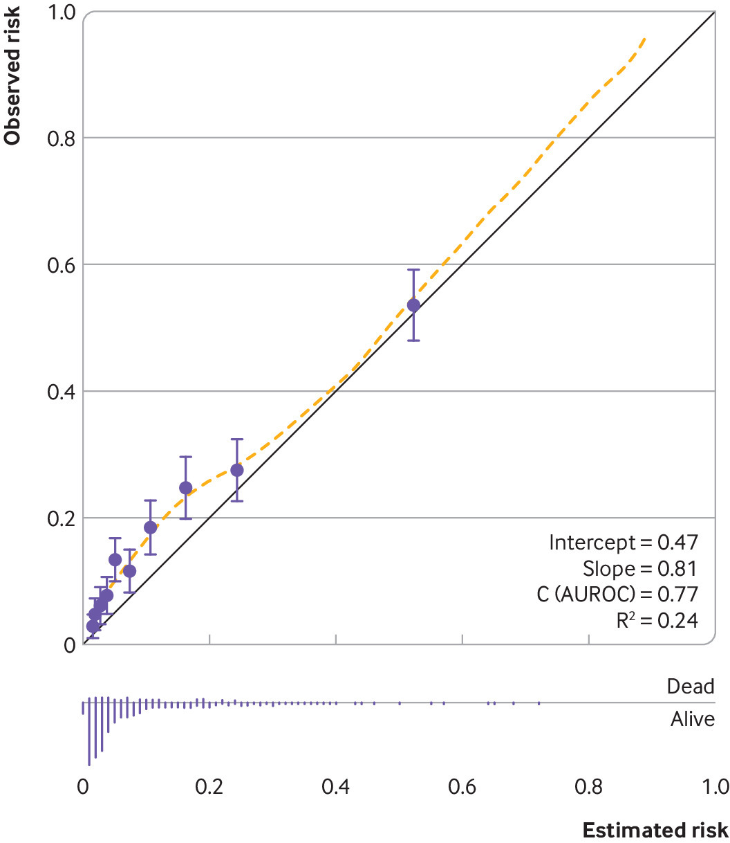
그림 3. 예측 모델에서 관찰된 위험과 추정된(예측된) 위험 사이의 일치를 조사하기 위한 교정 그림의 예. 이 연구는 파열된 두개내 동맥류로 인한 지주막하 출혈을 경험한 사람들의 사망 위험을 추정하기 위한 예측 모델을 개발했다. 원은 추정 위험의 10분의 1로 그룹화된 추정 및 관찰 위험이며, 노란색 점선은 추정 위험 범위에 걸친 일치를 포착하기 위해 황토색이 더 부드럽다. AUROC=수신 사업자 특성상 영역
Fig 3. Example of a calibration plot to examine agreement between observed risks and estimated (predicted) risks from a prediction model.64 The study developed prediction models to estimate the risk of mortality in individuals who experienced subarachnoid haemorrhage from ruptured intracranial aneurysm. Circles are estimated and observed risks grouped by 10ths of estimated risks, and the yellow dashed line is a loess smoother to capture agreement across the range of estimated risks. AUROC=area under the receiving operator characteristic
통계 편집자들은 또한 모델 개발 연구의 연구자들이 과적합 가능성을 줄이고 새로운 데이터의 예측 교정을 개선하는 데 도움이 되는 페널티화 또는 수축 방법(예: 능선 회귀, 라소, 탄성 그물)을 사용하여 재분석을 수행할 것을 제안할 수 있다. 퍼스 보정과 같은 처벌 방법은 데이터가 희박한 비예측 상황(예: 치료 효과를 추정하는 무작위 시험)에서도 중요할 수 있는데, 이 상황에서 표준 방법(로지스틱 회귀 분석과 같은)이 편향된 효과 추정치를 제공할 수 있기 때문이다.
Statistical editors may also suggest that researchers of model development studies undertake a reanalysis using penalisation or shrinkage methods (eg, ridge regression, lasso, elastic net), which reduce the potential for overfitting and help improve calibration of predictions in new data.6667 Penalisation methods, such as Firth’s correction,68 can also be important in non-prediction situations (eg, randomised trials estimating treatment effects) with sparse data, as standard methods (such as logistic regression) may give biased effect estimates in this situation.69
On the 10th day of Christmas, a statistician sent to me:
변수 선택 접근 방식을 신중하게 고려합니다
Carefully consider the variable selection approach
통계 검토에서 비판의 일반적인 영역은 변수 선택 방법(예: 효과의 통계적 유의성에 기초한 공변량 선택)의 사용이다. 이러한 방법을 사용하면 통계 편집자는 저자에게 정당성을 요청할 것이다. 연구에 따라, 통계 편집자들은 새해 첫날에 마지막으로 남은 칠면조 샌드위치처럼 저자들에게 이러한 접근법을 완전히 피하라고 제안할 수도 있다. 예를 들어, 일반적인 목표는 특정 요인이 [다른 (확립된) 예측 요인]에 비해 [예측 값을 추가하는 방법]에 대한 [편견 없는 추정치]를 제공하는 것이기 때문에 예측 요인 연구에서 변수 선택 방법을 가장 잘 피한다. 따라서 기존의 예측요인의 영향을 고려한 후 새로운 요인의 예측효과를 검토하기 위해서는 기존의 모든 요인에 강제적인 회귀모형이 필요하다. 마찬가지로, 관찰 데이터에 기초한 인과 연구에서 조정 요인으로 포함할 교란 요인의 선택은 인과 경로에 기초하여 선택되어야 한다 —예를 들어, 자동화된 선택 방법에 기초한 통계적 중요성이 아닌 (공변량과 결과 사이의 잠재적 매개자를 고려하여) 지시된 비순환 그래프를 사용하여 표현된다.
A common area of criticism in statistical reviews is the use of variable selection methods (eg, selection of covariates based on the statistical significance of their effects).70 If these methods are used, statistical editors will ask authors for justification. Depending on the study, statistical editors might even suggest authors avoid these approaches entirely, just as you would that last remaining turkey sandwich on New Year’s Day. For example, variable selection methods are best avoided in prognostic factor studies, as the typical aim is to provide an unbiased estimate of how a particular factor adds prognostic value over and above other (established) prognostic factors.71 Therefore, a regression model forcing in all the existing factors is needed to examine the prognostic effect of the new factor after accounting for the effect of existing prognostic factors. Similarly, in causal research based on observational data, the choice of confounding factors to include as adjustment factors should be selected based on the causal pathway—for example, as expressed using directed acyclic graphs (with consideration of potential mediators between covariates and outcome72), not statistical significance based on automated selection methods.
임상 예측 모델의 개발에서 잠재적 포함을 위한 모든 후보 예측 변수를 포함하는 전체 모델로 시작하는 라소 또는 탄성 네트와 같은 방법을 사용하여 변수 선택(수축을 통한)을 통합할 수 있다. 일반적이지만 부적절한 접근법은 예측 변수 포함에 대한 결정이 관측된 비조정 효과 추정치에 대한 P 값에 기초할 때 일변량 선별을 사용하는 것이다. 이것은 다른 예측 변수에 대한 조정 후 예측 변수의 효과이기 때문에 합리적인 전략이 아니다. 왜냐하면 실제로 관련 예측 변수는 (의료 전문가와 환자에 의해) 조합으로 사용되기 때문이다. 예를 들어, 재발 정맥 혈전 색전증의 위험에 대한 예후 모델을 개발하고 있을 때, 연구자들은 연령의 조정되지 않은 예후 효과가 일변량 분석에서 통계적으로 유의하지 않고 조정된 효과가 유의하며 다변량 분석과 반대 방향이라는 것을 발견했다.
In the development of clinical prediction models, variable selection (through shrinkage) may be incorporated using methods such as lasso or elastic net, which start with a full model including all candidate predictors for potential inclusion. A common, but inappropriate approach is to use univariable screening, when decisions for predictor inclusion are based on P values for observed unadjusted effect estimates. This is not a sensible strategy,73 as what matters is the effect of a predictor after adjustment for other predictors, because in practice the relevant predictors are used (by healthcare professionals and patients) in combination. When, for example, a prognostic model was being developed for risk of recurrent venous thromboembolism, the researchers found that the unadjusted prognostic effect of age was not statistically significant from univariable analysis but that the adjusted effect was significant and in the opposite direction from multivariable analysis.74
On the 11th day of Christmas, a statistician sent to me:
가정의 영향 평가
Assess the impact of any assumptions
모든 사람들은 그것이 크리스마스 영화라는 것에 동의하지만, 이것이 다이하드에 적용되는지는 논란의 여지가 있다. 마찬가지로 통계 편집자는 저자의 완고한 분석 가정에 대해 토론하고 가정이 변경될 경우 결과가 변경되는지 여부를 검토하도록 요청할 수 있다(감도 분석). 예를 들어, 재발까지의 시간이나 사망 시간과 같은 사건 발생 시간 데이터가 있는 제출된 시험에서는 위험 비율이 전체 추적 기간에 걸쳐 일정하다고 가정하여 보고하는 것이 일반적이다. 이 가정이 기사에서 정당화되지 않는 경우, 예를 들어 시간에 따라 위험 비율이 어떻게 변화하는지 그래픽으로 제시함으로써 저자들에게 이 문제를 해결하도록 요청할 수 있다. (아마도 관심 공변량과 (로그) 시간 사이의 상호작용을 포함하는 생존 모델에 기초한다.). 또 다른 예는 베이지안 분석을 사용한 제출물에서, 이전 분포는 "모호한" 또는 "비정보적"으로 분류되지만 여전히 영향력이 있을 수 있다. 이러한 상황에서 저자들은 다른 그럴듯한 사전 분포를 선택할 때 결과가 어떻게 변하는지 보여달라고 요청받을 수 있다.
Everyone agrees that It’s A Wonderful Life is a Christmas movie, but whether this applies to Die Hard is debatable. Similarly, statistical editors might debate authors’ die-hard analysis assumptions, and even ask them to examine whether results change if the assumptions change (a sensitivity analysis). For example, in submitted trials with time-to-event data, such as time to recurrence or death, it is common to report the hazard ratio, assuming it is a constant over the whole follow-up period. If this assumption is not justified in an article, authors may be asked to address this—for example, by graphically presenting how the hazard ratio changes over time (perhaps based on a survival model that includes an interaction between the covariate of interest and (log) time).75 Another example is in submissions with bayesian analyses, where prior distributions are labelled as “vague” or “non-informative” but may still be influential. In this situation, authors may be asked to demonstrate how results change when other plausible prior distributions are chosen.
On the 12th day of Christmas, a statistician sent to me:
보고 지침 사용 및 과도한 해석 방지
Use reporting guidelines and avoid overinterpretation
알트먼은 "독자들은 무엇이 행해졌는지 추론할 필요가 없어야 한다, 그것이 명확하게 말해져야 한다. 적절한 방법론이 사용되어야 하며 사용된 것으로 간주되어야 합니다." 불완전하게 보고된 연구는 변명의 여지가 없으며 크리스마스 트리 아래에 있는 라벨이 없는 선물과 마찬가지로 혼란을 일으킨다. 독자들은 보고된 연구의 근거와 목적, 연구 설계, 사용된 방법, 참가자 특성, 결과, 증거의 확실성, 연구 결과 등을 알아야 한다. 이러한 요소 중 하나라도 누락된 경우 저자는 이를 명확히 해야 합니다.
Altman once said, “Readers should not have to infer what was probably done, they should be told explicitly. Proper methodology should be used and be seen to have been used.”76 Incompletely reported research is indefensible and creates confusion, just as with those unlabelled presents under the Christmas tree. Readers need to know the rationale and objectives of a reported study, the study design, methods used, participant characteristics, results, certainty of evidence, research implications, and so forth. If any of these elements are missing, authors will be asked to clarify them.
보고 지침을 활용합니다. 그들은 보고할 항목의 체크리스트를 제공한다(산타는 이것을 두 번 확인할 것을 제안한다). 이 체크리스트는 독자(통계 편집자 포함)가 연구를 이해하고 그 결과를 비판적으로 평가할 수 있도록 하는데 필요한 최소한의 세부사항을 나타낸다. 보고 지침은 건강 연구 보고와 관련된 지침 및 기타 자료의 포괄적인 모음을 유지하는 EQUATOR 네트워크 웹 사이트에 나열되어 있습니다. 표 1은 무작위 시험을 위한 CONSTORT 문과 예측 모델 연구를 위한 TRIPOD 지침을 포함한 예를 보여준다. BMJ는 저자들에게 각 항목이 제출된 원고의 어느 페이지에 보고되었는지를 나타내는 관련 지침 내에 체크리스트를 작성하고 제출과 함께 포함할 것을 요구한다.
Make use of reporting guidelines. They provide a checklist of items to be reported (Santa suggests checking this twice), which represent the minimum detail required to enable readers (including statistical editors) to understand the research and critically appraise its findings. Reporting guidelines are listed on The EQUATOR Network website, which maintains a comprehensive collection of guidelines and other materials related to health research reporting.77Table 1 shows examples, including the CONSORT statement for randomised trials79 and the TRIPOD guideline for prediction model studies.8081The BMJ requires authors to complete the checklist within the relevant guideline (and include it with a submission), indicating on which page of the submitted manuscript each item has been reported.

보고와 관련된 통계 편집자 검토 과정의 또 다른 공통적인 부분은 인과관계, 결과의 일반화 가능성 또는 임상 실무에 대한 즉각적인 영향과 같은 결과의 해석을 지나치게 질의하는 것이다. 특히 다중 공변량(변수)이 있는 회귀 모델을 참조하기 위해 다변량(다변수가 아닌)을 오용하고, 그룹을 생성하는 데 사용되는 절단점이 아닌 그룹을 참조하기 위해 분위수를 오용하는 것(예: 십진법은 10개의 동일한 크기의 그룹을 생성하는 데 사용되는 9개의 절단점)을 오용한다업(10번째라고 함).
Another common part of the statistical editors review process, related to reporting, is to query overinterpretation of findings—and even spin,82 such as unjustified claims of causality, generalisability of results, or immediate implications for clinical practice. Incorrect terminology is another bugbear—in particular the misuse of multivariate (rather than multivariable) to refer to a regression model with multiple covariates (variables), and the misuse of quantiles to refer to groups rather than the cut points used to create the groups (eg, deciles are the nine cut points used to create 10 equal sized groups called 10ths).83
에피파니
Epiphany
BMJ에 제출된 기사의 동료 검토 중에 일상적으로 마주치는 12개의 통계 문제 목록은 향후 제출된 문서 작성자에게 도움이 될 것으로 기대된다. 지난 크리스마스 통계 편집자들은 이 목록을 트위터에 올렸지만, 어쨌든 그들은 다음날 제출이 저조했다. 올해, 그들을 눈물로부터 구하기 위해, 그들은 특별한 누군가를 위해 그것을 만들었습니다. 당신, BMJ 독자.
This list of 12 statistical issues routinely encountered during peer review of articles submitted to The BMJ will hopefully help authors of future submissions. Last Christmas statistical editors tweeted this list, but the very next day they got poor submissions anyway. This year, to save them from tears, they’ve tailored it for someone special—you, The BMJ reader.
저자들은 통계 검토 기간을 줄이고 통계 편집자들이 축제 기간 동안 중요한 (네, 말장난 의도로) 다른 사람들과 더 많은 시간을 보낼 수 있도록 함으로써 세상에 기쁨을 주기 위해 내년 크리스마스에 서둘러 논문을 제출하기 전에 이 목록을 다루어야 한다. 만약 저자들이 이 지침을 고수한다면, "크리스마스의 12번째 날에" 노래는 행복한 통계학자의 피드백을 반영한 가사와 함께 매우 긍정적인 "크리스마스 리뷰의 12번째 날에"로 바뀔 것이다(아마도 그림 4의 노래 시트 사용에 참여할 것이다).
Authors should address this list before rushing to submit papers to The BMJ next Christmas, in order to bring joy to the world by reducing the length of statistical reviews and allowing the statistical editors to spend more time with their significant (yes, pun intended) others over the festive period. If authors did adhere to this guidance, the “On the 12th Day of Christmas” song would change to the very positive “On the 12th Day of Christmas Review” with lyrics reflecting feedback from a happy statistician (perhaps join in using the song sheet in figure 4).
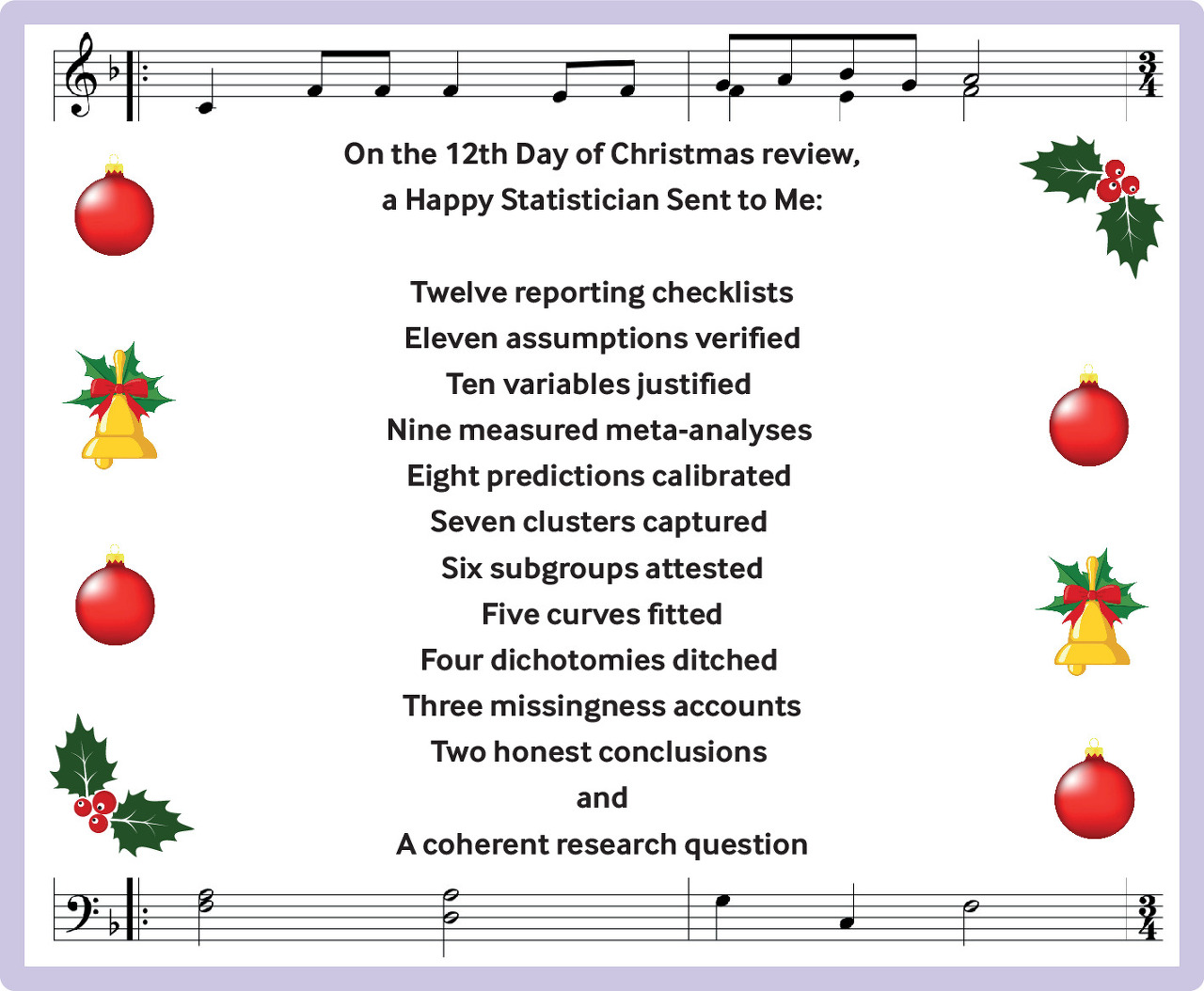
그림 4. "크리스마스 리뷰 12일째 되는 날, 행복한 통계학자가 나에게 보낸..."의 노래 시트
Fig 4. Song sheet for “On the 12th Day of Christmas Review, a Happy Statistician sent to me . . .”
궁극적으로, BMJ는 곰팡이가 아닌 금, 말도 안 되는 유향, 그리고 몰약을 출판하기를 원한다. 많은 다른 주제들이 언급될 수 있었고, 독자들은 더그 앨트먼과 마틴 블랜드가 작성한 BMJ Statistics Notes 시리즈, BMJ의 연구 방법 및 보고 섹션, 그리고 일반적인 통계 오류에 대한 다른 개요를 참조한다.
Ultimately, The BMJ wants to publish the gold not the mould, the frankincense not the makes-no-sense, and the myrrh not the urrgghh. Many other topics could have been mentioned, and for further guidance readers are directed to the BMJ Statistics Notes series (written mainly by Doug Altman and Martin Bland), the Research Methods and Reporting section of The BMJ,84 and other overviews of common statistical mistakes.8586
On the 12th Day of Christmas, a Statistician Sent to Me .
PMID: 36593578
'Articles (Medical Education) > 의학교육연구(Research)' 카테고리의 다른 글
| 양적연구 질문과 질적연구 질문 및 가설 작성의 실용 가이드 (J Korean Med Sci. 2022) (0) | 2023.03.04 |
|---|---|
| 주관적 평가를 측정할 때 동의-비동의 문항 사용의 재고(Res Social Adm Pharm. 2022) (0) | 2023.01.17 |
| 설문에서 최대한을 얻어내기: 응답 동기부여 최적화하기(J Grad Med Educ. 2022) (0) | 2023.01.15 |
| 구색만 갖추기: 어거지로 하는 설문이 자료 퀄리티에 미치는 영향(EDUCATIONAL RESEARCHER, 2021) (0) | 2023.01.15 |
| 의학교육의 패러다임, 가치론, 인간행동학 (Acad Med, 2018) (0) | 2022.11.13 |